23.4: Applications

Silico Detection Analysis

With the availability of such a powerful tool like FBA, more questions naturally arise. For example, are we able to predict gene knockout phenotype based on their simulated effects on metabolism? Also, why would we try to do this, even though other methods, like protein interaction map connective, exist? Such analysis is actually necessary, since other methods do not take into direct consideration the metabolic flux or other specific metabolic conditions.

source unknown. All rights reserved. This content is excluded from our Creative

Commons license. For more information, see http://ocw.mit.edu/help/faq-fair-use/.

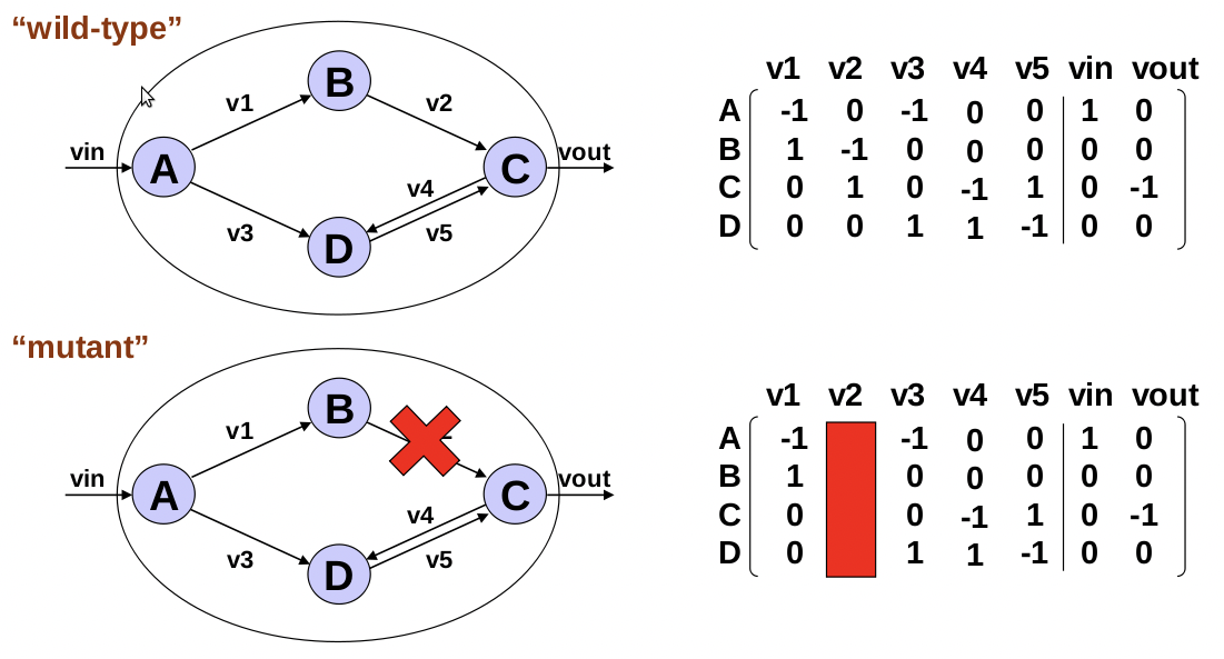
Figure 23.4: Removing a reaction is the same as removing a gene from the stoichiometric matrix.

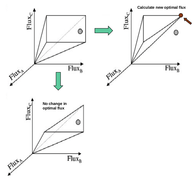
Knocking out a gene in an experiment is simply modeled by removing one of the columns (reactions) from the stochiometric matrix. (A question during class clarified that a single gene can knock out multiple columns/reactions.) Thereby, these knockout mutations will further constrain the feasible solution space by removing fluxes and their related extreme pathways. If the original optimal flux was outside is outside the new space, then new optimal flux is created. Thus the FBA analysis will produce different solutions. The solution is a maximal growth rate, which may be confirmed or disproven experimentally. The growth rate at the new solution provides a measure of the knockout phenotype. If these gene knockouts are in fact lethal, then the optimal solution will be a growth rate of zero.

Studies by Edwards, Palsson (1900) explore knockout phenotype prediction use to predict metabolic changes in response to knocking out enzymes in E. coli, a prokaryote [? ]. In other words, an in silico metabolic model of E.coli was constructed to simulate mutations affecting the glycolysis, pentose phosphate, TCA, and electron transport pathways (436 metabolites and 719 reactions included). For each specific condition, the optimal growth of mutants was compared to non-mutants. The in vivo and in silico results were then compared, with 86% agreement. The errors in the model indicate an underdeveloped model (lack of knowledge). The authors discuss 7 errors not modeled by FBA, including mutants inhibiting stable RNA synthesis and producing toxic intermediates.

source unknown. All rights reserved. This content is excluded from our Creative

Commons license. For more information, see http://ocw.mit.edu/help/faq-fair-use/.

Figure 23.5: Constraining the feasible solution space may create a new optimal flux.

Quantitative Flux In Silico Model Predictions

Can models quantitatively predict fluxes, growth rate? We demonstrate the ability of FBA to give quantitative predictions about growth rate and reaction fluxes given different environmental conditions. More specifically, prediction refers to externally measurable fluxes as a function of controlled uptake rates and environmental conditions. Since FBA maximizes an objective function, resulting in a specific value for this function, we should in theory be able to extract quantitative information from the model.

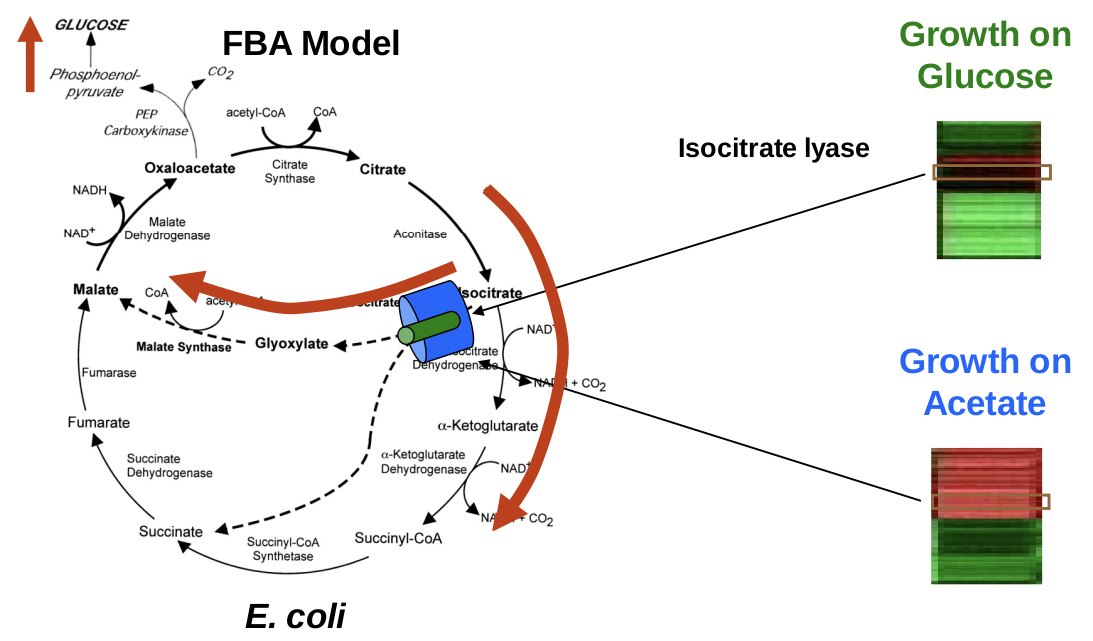
An early example by Edwards, Ibarra, and Palsson (1901), predicted the growth rate of E. coli in culture given a range of fixed uptake rates of oxygen and two carbon sources (acetate and succinate), which they could control in a batch reactor [6]. They assumed that E. coli cells adjust their metabolism to maximize growth (using a growth objective function) under given environmental conditions and used FBA to model the metabolic pathways in the bacterium. The input to this particular model is acetate and oxygen, which is labeled as VIN .

The controlled uptake rates fixed the values of the oxygen and acetate/succinate input fluxes into the network, but the other fluxes were calculated to maximize the value of the growth objective.

The growth rate is still treated as the solution to the FBA analysis. In sum, optimal growth rate is predicted as a function of uptake constraints on oxygen versus acetate and oxygen versus succinate. The basic model is a predictive line and may be confirmed in a bioreactor experimentally by measuring the uptake and growth from batch reactors (note: experimental uptake was not constrained, only measured).

This model by Palsson was the first good proof of principle in silico model. The authors quantitative growth rate predictions under the di↵erent conditions matched very closely to the experimentally observed growth rates, implying that E. coli do have a metabolic network that is designed to maximize growth. It had good true positive and true negative rates. The agreement between the predictions and experimental results is very impressive for a model that does not include any kinetic information, only stoichiometry. Prof. Galagan cautioned, however, that it is often dicult to know what good agreement is, because we dont know the significance of the size of the residuals. The organism was grown on a number of di↵erent nutrients. Therefore, the investigators were able to predict condition specific growth. Keep in mind this worked, since only certain genes are necessary for some nutrients, like fbp for gluconeogenesis. Therefore, knocking out fbp will only be lethal when there is no glucose in the environment, a specific condition that resulted in a growth solution when analyzed by FBA.

Quasi Steady State Modeling (QSSM)

We’re now able describe how to use FBA to predict time-dependent changes in growth rates and metabolite concentrations using quasi steady state modeling. The previous example used FBA to make quantitative growth predictions under specific environmental conditions (point predictions). Now, after growth and uptake fluxes, we move on to another assumption and type of model.

Can we use a steady state model of metabolism to predict the time-dependent changes in the cell or environments? We do have to make a number of quasi steady state assumptions (QSSA):

1. The metabolism adjusts to the environmental/cellular changes more rapidly than the changes themselves

2. The cellular and environmental concentrations are dynamic, but metabolism operates on the condition that the concentration is static at each time point (steady state model).

Is it possible to use QSSM to predict metabolic dynamics over time? For example, if there is less acetate being taken in on a per cell basis as the culture grows, then the growth rate must slow. But now, QSSA assumptions are applied. That is, in effect, at any given point in time, the organism is in steady state.

What values does one get as a solution to the FBA problem? There are fluxes the growth rate. We are predicting rate and fluxes (solution) where VIN/OUT included. Up to now we assumed that the input and output are infinite sinks and sources. To model substrate/growth dynamics, the analysis is performed a bit differently from prior quantitative flux analysis. We first divide time into slices t. At each time point t, we use FBA to predict cellular substrate uptake (Su) and growth (g) during interval t. The QSSA means these predictions are constant over t. Then we integrate to get the biomass (B) and substrate concentration (Sc) at the next time point t + t. Therefore, the new VIN is calculated each time based on points t in-between time. Thus we can predict the growth rate and glucose and acetate uptake (nutrients available in the environment). The four step analysis is:

1. The concentration at time is given by the substrate concentration from the last step plus any additional substrate provided to the cell culture by an inflow, such as in a fed batch.

2. The substrate concentration is scaled for time and biomass (X) to determine the substrate availability to the cells. This can exceed the maximum uptake rate of the cells or be less than that number.

3. Use the flux balance model to evaluate the actual substrate uptake rate, which may be more or less than the substrate available as determined by step 2.

4. The concentration for the next time step is then calculated by integrating the standard differential equations:

   \[\frac{d B}{d t}=g B \rightarrow B=B_{o} e^{g t}\nonumber]

   \[\frac{d S c}{d t}=-S u B \rightarrow S c=S c_{o} \frac{X}{g}\left(e^{g t}-1\right)\nonumber\]

The additional work by Varma et al. (1994) specifies the glucose uptake rate a priori [17]. The model simulations work to predict time-dependent changes in growth, oxygen uptake, and acetate secretion. This converse model plots uptake rates versus growth, while still achieving comparable results in vivo and in silico. The researchers used quasi steady state modeling to predict the time-dependent profiles of cell growth and metabolite concentrations in batch cultures of E. coli that had either a limited initial supply of glucose (left) or a slow continuous glucose supply (right diagram). A great fit is evident.

The diagrams above show the results of the model predictions (solid lines) and compare it to the experimental results (individual points). Thus, in E. coli, quasi steady state predictions are impressively accurate even with a model that does not account for any changes in enzyme expression levels over time. However, this model would not be adequate to describe behavior that is known to involve gene regulation. For example, if the cells had been grown on half-glucose/half-lactose medium, the model would not have been able to predict the switch in consumption from one carbon source to another. (This does occur experimentally when E. coli activates alternate carbon utilization pathways only in the absence of glucose.)

Regulation via Boolean Logic

There is a number of levels of regulation through which metabolic flux is controlled at the metabolite, transcriptional, translational, post-translational levels. FBA associated errors may be explained by incorporation of gene regulatory information into the models. One way to do this is Boolean logic. The following table describes if genes for associated enzymes are on or off in presence of certain nutrients (an example of incorporating E. coli preferences mentioned above):

ON no glucose(0)	ON acetate present(1)
ON glucose present(1)	OFF acetate present(1)

Therefore, one may think that the next step to take is to incorporate this fact into the models. For example, if we have glucose in the environment, the acetate processing related genes are off and therefore absent from the S matrix which now becomes dynamic as a result of incorporation of regulation into our model. In the end, our model is not quantitative. The basic regulation then describes that if one nutrient- processing enzyme is on, the other is off. Basically it is a bunch of Boolean logic, based on presence of enzymes, metabolites, genes, etc. These Boolean style assumptions are then used at every small change in time dt to evaluate the growth rate, the fluxes, and such variables. Then, given the predicted fluxes, the VIN ,the VOUT , and the system states, one can use logic to turn genes off and on, effectively a S per t. We can start putting together all of the above analyses and come up with a general approach in metabolic modeling. We can tell that if glycolysis is on, then gluconeogenesis must be off.

The first attempt to include regulation in an FBA model was published by Covert, Schilling, and Palsson in 1901 [7]. The researchers incorporated a set of known transcriptional regulatory events into their analysis of a metabolic regulatory network by approximating gene regulation as a Boolean process. A reaction was said to occur or not depending on the presence of both the enzyme and the substrate(s): if either the enzyme that catalyzes the reaction (E) is not expressed or a substrate (A) is not available, the reaction flux will be zero:

rxn = IF (A) AND (E)

Similar Boolean logic determined whether enzymes were expressed or not, depending on the currently ex- pressed genes and the current environmental conditions. For example, transcription of the enzyme (E) occurs only if the appropriate gene (G) is available for transcription and no repressor (B) is present:

trans = IF (G) AND NOT (B)

The authors used these principles to design a Boolean network that inputs the current state of all relevant genes (on or off) and the current state of all metabolites (present or not present), and outputs a binary vector containing the new state of each of these genes and metabolites. The rules of the Boolean network were constructed based on experimentally determined cellular regulatory events. Treating reactions and enzyme/metabolite concentrations as binary variables does not allow for quantitative analysis, but this method can predict qualitative shifts in metabolic fluxes when merged with FBA. Whenever an enzyme is absent, the corresponding column is removed from the FBA reaction matrix, as was described above for knockout phenotype prediction. This leads to an iterative process:

1. Given the initial states of all genes and metabolites, calculate the new states using the Boolean network;

2. perform FBA with appropriate columns deleted from the matrix, based on the states of the enzymes, to determine the new metabolite concentrations;

3. repeat the Boolean network calculation with the new metabolite concentrations; etc. The above model is not quantitative, but rather a pure simulation of turning genes on and off at any particular time instant.

On a few metabolic reactions, there are rules about allowing organism to shift carbon sources (C1, C2).

An application of this method from the study by Covert et al.[7] was to simulate diauxic shift, a shift from metabolizing a preferred carbon source to another carbon source when the preferred source is not available. The modeled process includes two gene products, a regulatory protein RPc1, which senses (is activated by) Carbon 1, and a transport protein Tc2, which transports Carbon 2. If RPc1 is activated by Carbon 1, Tc2 will not be transcribed, since the cell preferentially uses Carbon 1 as a carbon source. If Carbon 1 is not available, the cell will switch to metabolic pathways based on Carbon 2 and will turn on expression of Tc2.

The Booleans can represent this information:

RPc1 = IF(Carbon1) Tc2 = IF NOT(RPc1)

Covert et al. found that this approach gave predictions about metabolism that matched results from experimentally induced diauxic shift. This diauxic shift is well modeled by the in silico analysis see above figure. In segment A, C1 is used up as a nutrient and there is growth. In segment B, there is no growth as C1 has run out and C2 processing enzymes are not yet made, since genes have not been turned on (or are in the process), thus the delay of constant amount of biomass. In segment C, enzymes for C2 turned on and the biomass increases as growth continues with a new nutrient source. Therefore, if there is no C1, C2 is used up. As C1 runs out, the organism shifts metabolic activity via genetic regulation and begins to take up C2. Regulation predicts diauxie, the use of C1 before C2. Without regulation, the system would grow on both C1 and C2 together to max biomass.

So far we have discussed using this combined FBA-Boolean network approach to model regulation at the transcriptional/translational level, and it will also work for other types of regulation. The main limitation is for slow forms of regulation, since this method assumes that regulatory steps are completed within a single time interval (because the Boolean calculation is done at each FBA time step and does not take into account previous states of the system). This is fine for any forms of regulation that act at least as fast as transcription/translation. For example, phosphorylation of enzymes (an enzyme activation process) is very fast and can be modeled by including the presence of a phosphorylase enzyme in the Boolean network.

However, regulation that occurs over longer time scales, such as sequestration of mRNA, is not taken into account by this model. This approach also has a fundamental problem in that it does not allow actual experimental measurements of gene expression levels to be inputted at relevant time points.

We do not need our simulations to artificially predict whether certain genes are on or off. Microarray expression data allows us to determine which genes are being expressed, and this information can be incorporated into our models.

Coupling Gene Expression with Metabolism

In practice, we do not need to artificially model gene levels, we can measure them. As discussed previousky, it is possible to measure the expressions levels of all the mRNAs in a given sample. Since mRNA expression data correlates with protein expression data, it would be extremely useful to incorporate it into the FBA. Usually, data from microarray experiments is clustered, and unknown genes are hypothesised to have function similar to the function of those known genes with which they cluster. This analysis can be faulty, however, as genes with similar actions may not always cluster together. Incorporating microarray expression data into FBA could allow an alternate method of interpretation of the data. Here arises a question, what is the relationship between gene level and flux through a reaction?

Say the reaction A ! B is catalyzed by an enzyme. If a lot of A present, increased expression of the gene for the enzyme causes increased reaction rate. Otherwise, increasing gene expression level will not increase reaction rate. However, the enzyme concentration can be treated as a constraint on the maximum possible flux, given that the substrate also has a reasonable physiological limit.

The next step, then, is to relate the mRNA expression level to the enzyme concentration. This is more dicult, since cells have a number of regulatory mechanisms to control protein concentrations independently of mRNA concentrations. For example, translated proteins may require an additional activation step (e.g. phosphorylation), each mRNA molecule may be translated into a variable number of proteins before it is degraded (e.g. by antisense RNAs), the rate of translation from mRNA into protein may be slower than the time intervals considered in each step of FBA, and the protein degradation rate may also be slow. Despite these complications, the mRNA expression levels from microarray experiments are usually taken as upper bounds on the possible enzyme concentrations at each measured time point. Given the above relationship between enzyme concentration and flux, this means that the mRNA expression levels are also upper bounds on the maximum possible fluxes through the reactions catalyzed by their encoded proteins. The validity of this assumption is still being debated, but it has already performed well in FBA analyses and is consistent with recent evidence that cells do control metabolic enzyme levels primarily by adjusting mRNA levels. (In 1907, Professor Galagan discussed a study by Zaslaver et al. (1904) that found that genes required in an amino acid biosynthesis pathway are transcribed sequentially as needed [2]). This is a particularly useful assumption for including microarray expression data in FBA, since FBA makes use of maximum flux values to constrain the flux balance cone.

Colijn et al. address the question of algorithmic integration of expression data and metabolic networks [3]. They apply FBA to model the maximum flux through each reaction in a metabolic network. For example, if microarray data is available from an organism growing on glucose and from an organism growing on acetate, significant regulatory di↵erences will likely be observed between the two datasets. Vmax tells us what the maximum we can reach. Microarray detects the level of transcripts, and it gives an upper boundary of Vmax.

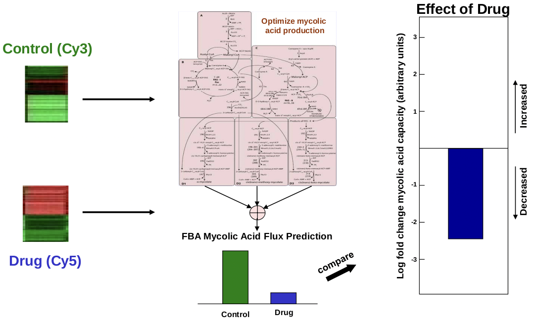
In addition to predicting metabolic pathways under different environmental conditions, FBA and microarray experiments can be combined to predict the state of a metabolic system under varying drug treatments. For example, several TB drugs target mycolic acid biosynthesis. Mycolic acid is a major cell wall constituent. In a 1904 paper by Bosho↵ et al., researchers tested 75 drugs, drug combinations, and growth conditions to

Figure 23.6: Model of Coljin et. al [3]

Courtesy of the authors. License: CC BY.

Source: Colijin, Caroline, et al. "Interpreting Expression Data with Metabolic Flux Models: Predicting Mycobacterium

Tubercluosis Mycolic acid Production." PLoS Computational Biology 5, no. 8 (2009): e1000489

see what effect different treatments had on mycolic acid synthesis [9]. In 1905, Raman et al. published an FBA model of mycolic acid biosynthesis, consisting of 197 metabolites and 219 reactions [13].

The basic flow of the prediction was to take a control expression value and a treatment expression value for a particular set of genes, then feed this information into the FBA and measure the final effect on the treatment on the production of mycolic acid. To examine predicted inhibitors and enhancers, they examined significance, which examines whether the effect is due to noise, and specificity, which examines whether the effect is due to mycolic acid or overall supression/enhancement of metabolism. The results were fairly encouraging. Several known mycolic acid inhibitors were identified by the FBA. Interesting results were also found among drugs not specifically known to inhibit mycolic acid synthesis. 4 novel inhibitors and 2 novel enhancers of mycolic acid synthesis were predicted. One particular drug, Triclosan, appears to be an enhancer according to the FBA model, whereas it is currently known as an inhibitor. Further study of this particular drug would be interesting. Experimental testing and validation are currently in progress.

Clustering may also be ineffective in identifying function of various treatments. Predicted inhibitors, and predicted enhancers of mycolic acid synthesis are not clustered together. In addition, no labeled training set is required for FBA-based algorithmic classification, whereas it is necessary for supervised clustering algorithms.

Predicting Nutrient Source

Now, we get the idea of predicting the nutrient source that an organism may be using in an environment, by looking at expression data and looking for associated nutrient processing gene expression. This is easier, since we cant go into the environment and measure all chemical levels, but we can get expression data rather easily. That is, we try to predict a nutrient source through predictions of metabolic state from expression data, based on the assumption that organisms are likely to adjust metabolic state to available nutrients. The nutrients may then be ranked by how well they match the metabolic states.

The other way around could work too. Can I predict a nutrient given a state? Such predictions could be useful for determining the nutrient requirements of an organism with an unknown natural environment, or for determining how an organism changes its environment. (TB, for example, is able to live within the environment of a macrophage phagolysosome, presumably by altering the environmental conditions in the

Figure 23.7: Basic flow in predicting state of a metabolic system under varing drug treatments phagolysosome and preventing its maturation.)

Courtesy of the authors. License: CC BY.

Source: Coljin, Caroline, et al. "Interpreting Expression Data with Metabolic Flux Models: Predicting

Mycobacterium Tuberculosis Mycolic Acid Production." PLoS Computational Biology 5, no. 8 (2009): e1000489

We can use FBA to define a space of possible metabolic states and choose one. The basic steps are to:

• Start with max flux cone (representing best growth with all nutrients available in environment). Find optimal flux for each nutrient.

• Apply expression data set (still not knowing nutrient). This will allow you to constrain the cone shape and figure out the nutrient, which is represented as one with the closest distance to optimal solution.

source unknown. All rights reserved. This content is excluded from our Creative

Commons license. For more information, see http://ocw.mit.edu/help/faq-fair-use/.

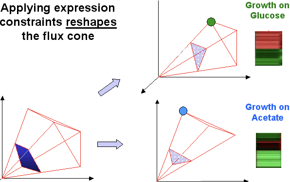
Figure 23.8: Applying expression data set allows constraining of cone shape.

In Figure 8, you may see that the first cone has a number of optimals, so the real nutrient is unknown. However, after expression data is applied, the cone is reshaped. It has only one optimal, which is still in feasible space and thereby must be that nutrient you are looking for.

As before, the measured expression levels provide constraints on the reaction fluxes, altering the shape of the flux-balance cone (now the expression-constrained flux balance cone). FBA can be used to determine the optimal set of fluxes that maximize growth within these expression constraints, and this set of fluxes can be compared to experimentally-determined optimal growth patterns under each environmental condition of interest. The difference between the calculated state of the organism and the optimal state under each condition is a measure of how sub-optimal the current metabolic state of the organism would be if it were in fact growing under that condition.

source unknown. All rights reserved. This content is excluded from our Creative

Commons license. For more information, see http://ocw.mit.edu/help/faq-fair-use/.

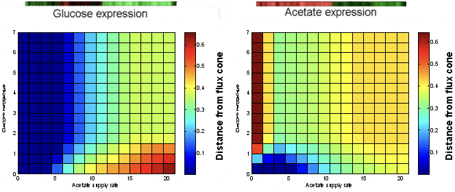
Figure 23.9: Results of nutrient source prediction experiment.

Expression data from growth and metabolism may then be applied to predict the carbon source being used. For example, consider E. coli nutrient product. We can simulate this system for glucose versus acetate. The color indicates the distance from the constrained flux cone to the optimal flux solution for that nutrient combo (same procedure described above). Then, multiple nutrients may be ranked, prioritized according to expression data. Unpublished data from Desmond Lun and Aaron Brandes provide an example of this approach.

They used FBA to predict which nutrient source E. coli cultures were growing on, based on gene expression data. They compared the known optimal fluxes (the optimal point in flux space) for each nutrient condition to the allowed optimal flux values within the expression-constrained flux-balance cone. Those nutrient conditions with optimal fluxes that remained within (or closest to) the expression-constrained cone were the most likely possibilities for the actual environment of the culture.

Results of the experiment are shown in Figure 9, where each square in the results matrices is colored based on the distance between the optimal fluxes for that nutrient condition and the calculated optimal fluxes based on the expression data. Red values indicate large distances from the expression-constrained flux cone and blue values indicate short distances from the cone. In the glucose-acetate experiments, for example, the results of the experiment on the left indicate that low acetate conditions are the most likely (and glucose was the nutrient in the culture) and the results of the experiment on the right indicate that low glucose/medium acetate conditions are the most likely (and acetate was the nutrient in the culture). When 6 possible nutrients were considered, the model always predicted the correct one, and when 18 possible nutrients were considered, the correct one was always one of the top 4 ranking predictions. These results suggest that it is possible to use expression data and FBA modeling to predict environmental conditions from information about the metabolic state of an organism.

This is important because TB uses fatty acids in macrophages in immune systems. We do not know which ones exactly are utilized. We can figure out what the TB sees in its environment as a food source and proliferation factor by analyzing what related nutrient processing genes are turned on at growth phases and such. Thereby we can figure out the nutrients it needs to grow, allowing for a potential way to kill it off by not supplying such nutrients or knocking out those particular genes.

It is easier to get expression data to see flux activity than see whats being used up in the environment by analyzing the chemistry on such a tiny level. Also, we might not be able to grow some bacteria in lab, but we can solve the problem by getting the expression data from the bacteria growing in a natural environment and then seeing what it is using to grow. Then, we can add it to the laboratory medium to grow the bacteria successfully.