23.3: Metabolic Flux Analysis

Metabolic flux analysis (MFA) is a way of computing the distribution of reaction fluxes that is possible in a given metabolic network at steady state. We can place constraints on certain fluxes in order to limit the space described by the distribution of possible fluxes. In this section, we will develop a mathematical formulation for MFA. Once again, this analysis is independent of the particular biology of the system; rather, it will only depend on the (universal) stoichiometries of the reactions in question.

Mathematical Representation

Consider a system with m metabolites and n reactions. Let xi be the concentration of substrate i, so that the rate of change of the substrate concentration is given by the time derivative of xi . Let x be the column vector (with m components) with elements xi . For simplicity, we consider a system with m = 4 metabolites A, B, C, and D. This system will consist of many reactions between these metabolites, resulting in a complicated balance between these compounds.

Once again, consider the simple reaction A + 2B \(\rightarrow\) 3C. We can represent this reaction in vector form as (-1 -2 3 0). Note that the first two metabolites (A and B) have negative signs, since they are consumed in the reaction. Moreover, the elements of the vector are determined by the stoichiometry of the reaction, as in Section 2.1. We repeat this procedure for each reaction in the system. These vectors become the columns of the stoichiometric matrix S. If the system has m metabolites and n reactions, S will be a m n matrix. Therefore, if we define v to be the n-component column vector of fluxes in each reaction, the vector S_v describes the rate of change of the concentration of each metabolite. Mathematically, this can be represented as the fundamental equation of metabolic flux analysis:

\[\frac{d x}{d t}=S v\nonumber\]

The matrix S is an extraordinarily powerful data structure that can represent a variety of possible scenarios in biological systems. For example, if two columns c and d of S have the property that c = d, the columns represent a reversible reaction. Moreover, if a column has the property that only one component is nonzero, it represents in exchange reaction, in which there is a flux into (or from) a supposedly infinite sink (or source), depending on the sign of the nonzero component.

We now impose the steady state assumption, which says that the left size of the above equation is identically zero. Therefore, we need to find vectors v that satisfy the criterion S_v = 0. Solutions to this equation will determine feasible fluxes for this system.

Null Space of S

The feasible flux space of the reactions in the model system is defined by the null space of S, as seen above. Recall from elementary linear algebra that the null space of a matrix is a vector space; that is, given two vectors y and z in the nullspace, the vector ay + bz (for real numbers a, b) is also in the null space. Since the null space is a vector space, there exists a basis bi, a set of vectors that is linearly independent and spans the null space. The basis has the property that for any flux v in the null space of S, there exist real numbers \(\alpha\)_i such that

\[v=\Sigma_{i} \alpha_{i} b_{i}\nonumber\]

How do we find a basis for the null space of a matrix? A useful tool is the singular value decomposition (SVD) [4]. The singular value decomposition of a matrix S is defined as a representation S = UEV*, where U is a unitary matrix of size m, V is a unitary matrix of size n, and E is a mxn diagonal matrix, with the (necessarily positive) singular values of S in descending order. (Recall that a unitary matrix is a matrix with orthonormal columns and rows, i.e. U * U = U U * = I the identity matrix). It can be shown that any matrix has an SVD. Note that the SVD can be rearranged into the equation \(S v=\sigma u\), where u and v are columns of the matrices U and V and is a singular value. Therefore, if \(\sigma\) = 0, v belongs to the null space of S. Indeed, the columns of V that correspond to the zero singular values form an orthonormal basis for the null space of S. In this manner, the SVD allows us to completely characterize the possible fluxes for the system.

Constraining the Flux Space

The first constraint mentioned above is that all steady-state flux vectors must be in the null space. Also negative fluxes are not thermodynamically possible. Therefore a fundamental constraint is that all fluxes must be positive. (Within this framework we represent reversible reactions as separate reactions in the stoichiometric matrix S having two unidirectional fluxes.)

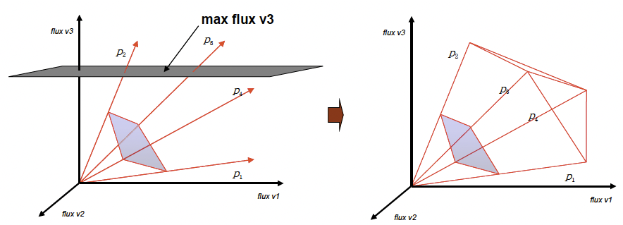
These two key constraints form a system that can be solved by convex analysis. The solution region can be described by a unique set of Extreme Pathways. In this region, steady state flux vectors v can be described as a positive linear combination of these extreme pathways. The Extreme Pathways, represented in slide 25 as vectors bi, circumscribe a convex flux cone. Each dimension is a rate for some reaction. In slide 25, the z-dimension represents the rate of reaction for v3 . We can recognize that at any point in time, the organism is living at a point in the flux cone, i.e. is demonstrating one particular flux distribution. Every point in the flux cone can be described by a possible steady state flux vector, while points outside the cone cannot.

One problem is that the flux cone goes out to infinity, while infinite fluxes are not physically possible. Therefore an additional constraint is capping the flux cone by determining the maximum fluxes of any of our reactions (these values correspond to our Vmax parameters). Since many metabolic reactions are interior to the cell, there is no need to set a cap for every flux. These caps can be determined experimentally by measuring maximal fluxes, or calculated using mathematical tools such as diffusivity rules.

We can also add input and output fluxes that represent transport into and out of our cells (Vin and Vout). These are often much easier to measure than internal fluxes and can thus serve to help us to generate a more biologically relevant flux space. An example of an algorithm for solving this problem is the simplex algorithm [1]. Slides 24-27 demonstrate how constraints on the fluxes change the geometry of the flux cone. In reality, we are dealing with problems in higher dimensional spaces.

Figure 23.2: Adding constraints to extreme pathways.

Linear Programming

Linear programming is a generic solution that is capable of solving optimization problems given linear constraints. These can be represented in a few different forms.

Canonical Form :

• Maximize: \(c^{T} x\)
• Subject to: \(A x \leq b\)

Standard Form :

• Maximize \(\Sigma c_{i} * x_{i}\)
• Subject to \(a_{i j} X_{i} \leq b_{i} \text { foralli, } j\)
• Non-negativity constraint: \(X_{i} \geq 0\)

A concise and clear introduction to Linear Programming is available here: www.purplemath. com/modules/linprog.htm The constraints described throughout section 3 give us the linear programming problem described in lecture. Linear programming can be considered a first approximation and is a classic problem in optimization. In order to try and narrow down our feasible flux, we assume that there exists a fitness function which is a linear combination of any number of the fluxes in the system. Linear programming (or linear optimization) involves maximizing or minimizing a linear function over a convex polyhedron specified by linear and non-negativity constraints.

Figure 23.3: Maximizing two functions with linear programming.

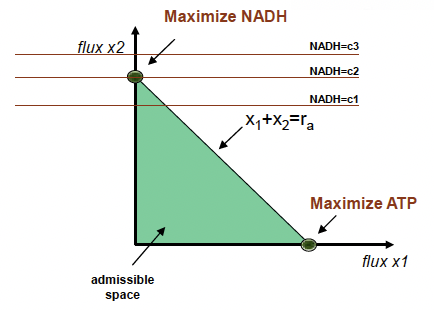
We solve this problem by identifying the flux distribution that maximizes an objective function:

The key point in linear programming is that our solutions lie at the boundaries of the permissible flux space and can be on points, edges, or both. By definition however, an optimal solution (if one exists) will lie at a point of the permissible flux space. This concept is demonstrated on slide 30. In that slide, A is the stoichiometric matrix, x is the vector of fluxes, and b is a vector of maximal permissible fluxes.

Linear programs, when solved by hand, are generally done by the Simplex method. The simplex method sets up the problem in a matrix and performs a series of pivots, based on the basic variables of the problem statement. In worst case, however, this can run in exponential time. Luckily, if a computer is available, two other algorithms are available. The ellipsoid algorithm and Interior Point methods are both capable of solving any linear program in polynomial time. It is interesting to note, that many seemingly dicult problems can be modeled as linear programs and solved eciently (or as eciently as a generic solution can solve a specific problem).

In microbes such as E. coli, this objective function is often a combination of fluxes that contributes to biomass, as seen in slide 31. However, this function need not be completely biologically meaningful.

For example, we might simulate the maximization of mycolates in M. tuberculosis, even though this isnt happening biologically. It would give us meaningful predictions about what perturbations could be performed in vitro that would perturb mycolate synthesis even in the absence of the maximization of the production of those metabolites.Flux balance analysis (FBA) was pioneered by Palssons group at UCSD and has since been applied to E. coli, M. tuberculosis, and the human red blood cell [? ].