17.4: Gibbs Sampling- Sample from joint (M,Zij) distribution

Last updated
Save as PDF

Page ID: 41017

\( \newcommand{\vecs}[1]{\overset { \scriptstyle \rightharpoonup} {\mathbf{#1}} } \) \( \newcommand{\vecd}[1]{\overset{-\!-\!\rightharpoonup}{\vphantom{a}\smash {#1}}} \)\(\newcommand{\id}{\mathrm{id}}\) \( \newcommand{\Span}{\mathrm{span}}\) \( \newcommand{\kernel}{\mathrm{null}\,}\) \( \newcommand{\range}{\mathrm{range}\,}\) \( \newcommand{\RealPart}{\mathrm{Re}}\) \( \newcommand{\ImaginaryPart}{\mathrm{Im}}\) \( \newcommand{\Argument}{\mathrm{Arg}}\) \( \newcommand{\norm}[1]{\| #1 \|}\) \( \newcommand{\inner}[2]{\langle #1, #2 \rangle}\) \( \newcommand{\Span}{\mathrm{span}}\) \(\newcommand{\id}{\mathrm{id}}\) \( \newcommand{\Span}{\mathrm{span}}\) \( \newcommand{\kernel}{\mathrm{null}\,}\) \( \newcommand{\range}{\mathrm{range}\,}\) \( \newcommand{\RealPart}{\mathrm{Re}}\) \( \newcommand{\ImaginaryPart}{\mathrm{Im}}\) \( \newcommand{\Argument}{\mathrm{Arg}}\) \( \newcommand{\norm}[1]{\| #1 \|}\) \( \newcommand{\inner}[2]{\langle #1, #2 \rangle}\) \( \newcommand{\Span}{\mathrm{span}}\)\(\newcommand{\AA}{\unicode[.8,0]{x212B}}\)

Sampling motif positions based on the Z vector

Gibbs sampling is similar to EM except that it is a stochastic process, while EM is deterministic. In the expectation step, we only consider nucleotides within the motif window in Gibbs sampling. In the maximization step, we sample from Z_ij and use the result to update the PWM instead of averaging over all values as in EM.

Step 1: Initialization As with EM, you generate your initial PWM with a random sampling of initial starting positions. The main difference lies in the Maximization step. During EM, the algorithm creates the sequence motif by considering all possible starting points of the motif. During Gibbs, the algorithm picks a single starting point of the motif with the probability of the starting points Z.

Step 2: Remove Remove one sequence, Xi, from your set of sequences. You will change the starting location of for this particular sequence.

Step 3: Update Using the remaining set of sequences, update the PWM by counting how often each base occurs in each position, adding pseudocounts as necessary.

Step 4: Sample Using the newly updated PWM, compute the score of each starting point in the sequence Xi. To generate each score, Zij, the following formula is used:

\[ A_{i j}=\frac{\prod_{k=j}^{j+W-1} p_{e k}, k-j+1}{\prod_{k=j}^{j+W-1} p_{c k}, 0} \nonumber \]

This is simply the probability that the sequence was generated using the motif PWM divided by the probability that the sequence was generated using the background PWM.

Select a new starting position for X_i by randomly choosing a position based on its Z_ij.

Step 5: Iterate Loop back to Step 2 and iterate the algorithm until convergence.

More likely to find global maximum, easy to implement

Because Gibbs updates its sequence motif during Maximization based of a single sample of the Motif rather than every sample weighted by their scores, Gibbs is less dependent on the starting PWM. EM is much more likely to get stuck on a local maximum than Gibbs because of this fact. However, this does not mean that Gibbs will always return the global maximum. Gibbs must be run multiple times to ensure that you have found the global maximum and not the local maximum.Two popular implementations of Gibbs Sampling applied to this problem are AlignACE and BioProspector. A more general Gibbs Sampler can be found in the program WinBUGS. Both AlignACE and BioProspector use the aforementioned algorithm for several choices of initial values and then report common motifs. Gibbs sampling is easier to implement than E-M, and in theory, it converges quickly and is less likely to get stuck at a local optimum. However, the search is less systematic.

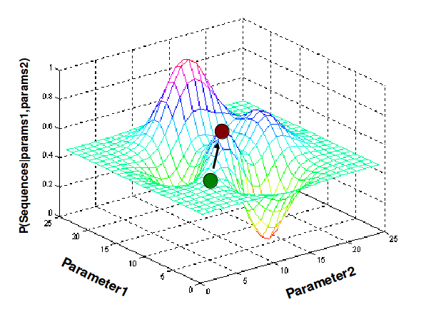
© source unknown. All rights reserved. This content is excluded from our Creative Commons license. For more information, see http://ocw.mit.edu/help/faq-fair-use/.
Figure 17.6: Gibbs Sampling