17.3: Expectation maximization

The key idea behind EM

We are given a set of sequences with the assumption that motifs are enriched in them. The task is to find the common motif in those sequences. The key idea behind the following probabilistic algorithms is that if we were given motif starting positions in each sequence, finding the motif PWM would be trivial; similarly, if we were given the PWM for a particular motif, it would be easy to find the starting positions in the input sequences. Let Z be the matrix in which Z_ij corresponds to the probability that a motif instance starts at position j in sequence i (a graphical of the probability distributions summarized in Z is shown in Figure 17.8). These algorithms therefore rely on a basic iterative approach: given a motif length L and an initial matrix Z, we can use the starting positions to estimate the motif, and in turn use the resulting motif to re-estimate the starting positions, iterating over these two steps until convergence on a motif.

© source unknown. All rights reserved. This content is excluded from our Creative Commons license. For more information, see http://ocw.mit.edu/help/faq-fair-use/.

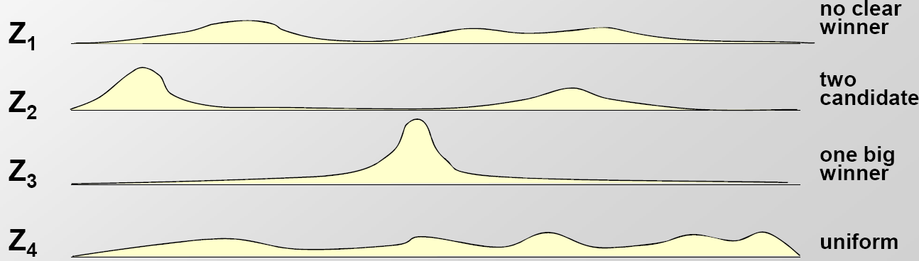
Figure 17.3: Examples of the Z matrix computed

The E step: Estimating Z_ij from the PWM

© source unknown. All rights reserved. This content is excluded from our Creative Commons license. For more information, see http://ocw.mit.edu/help/faq-fair-use/.

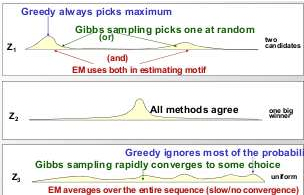
Figure 17.4: Selecting motif location: the greedy algorithm will always pick the most probable location for the motif. The EM algorithm will take an average while Gibbs Sampling will actually use the probability distribution given by Z to sample a motif in each step

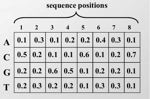
Step 1: Initialization The first step in EM is to generate an initial probability weight matrix (PWM). The PWM describes the frequency of each nucleotide at each location in the motif. In 17.5, there is an example of a PWM. In this example, we assume that the motif is eight bases long.

If you are given a set of aligned sequences and the location of suspected motifs within them, then finding the PWM is accomplished by computing the frequency of each base in each position of the suspected motif. We can initialize the PWM by choosing starting locations randomly.

We refer to the PWM as p_ck, where p_ck is the probability of base c occurring in position k of the motif. Note: if there is 0 probability, it is generally a good idea to insert pseudo- counts into your probabilities. The PWM is also called the profile matrix. In addition to the PWM, we also keep a background distribution p_ck,k=0, a distribution of the bases not in the motif.

Step 2: Expectation In the expectation step, we generate a vector Zij which contains the probability of the motif starting in position j in sequence i. In EM, the Z vector gives us a way of classifying all of the nucleotides in the sequences and tell us whether they are part of the motif or not. We can calculate Z_ij using Bayes’ Rule. This simplifies to:

\[ Z_{i j}^{t}=\frac{\operatorname{Pr}^{t}\left(X_{i} \mid Z_{i j}\right) \operatorname{Pr}^{t}\left(Z_{i j}=1\right)}{\Sigma_{k=1}^{L-W+1} \operatorname{Pr}^{t}\left(X_{i} \mid Z_{i j}=1\right) \operatorname{Pr}^{t}\left(Z_{i k}=1\right)} \nonumber \]

Figure 17.5: Sample position weight matrix

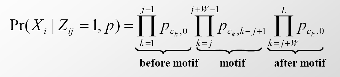
where \(\operatorname{Pr}^{t}\left(X_{i} \mid Z_{i j}=1\right)=\operatorname{Pr}\left(X_{i} \mid Z_{i j}=1, p\right)\) is defined as

This is the probability of sequence i given that the motif starts at position j. The first and last products correspond to the probability that the sequences preceeding and following the candidate motif come from some background probability distribution whereas the middle product corresponds to the probability that the candidate motif instance came from a motif probability distribution. In this equation, we assume that the sequence has length L and the motif has length W .

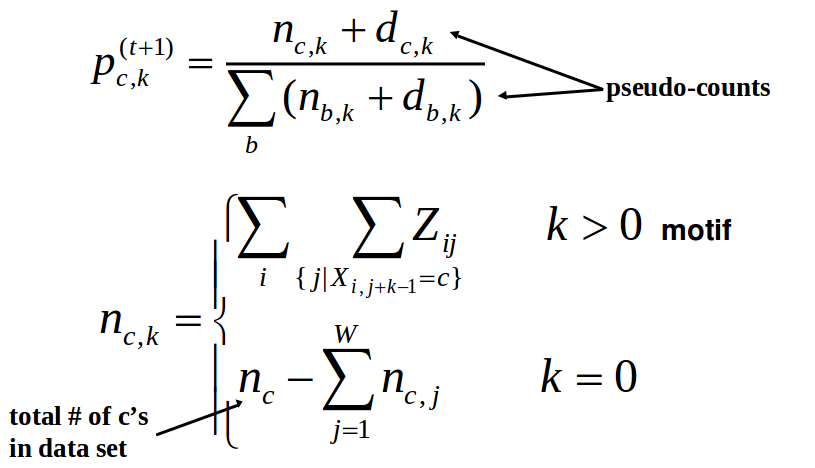
step: Finding the maximum likelihood motif from starting positions Zij

Step 3: Maximization Once we have calculated Zt, we can use the results to update both the PWM and the background probability distribution. We can update the PWM using the following equation

Figure \(\PageIndex{1}\): Copy and Paste Caption here. (Copyright; author via source)

Step 4: Repeat Repeat steps 2 and 3 until convergence.

One possible way to test whether the profile matrix has converged is to measure how much each element in the PWM changes after step maximization. If the change is below a chosen threshold, then we can terminate the algorithm. EM is a deterministic algorithm and is entirely dependent on the initial starting points because it uses an average over the full probability distribution. It is therefore advisable to rerun the algorithm with different intial starting positions to try reduce the chance of converging on a local maximum that is not the global maximum and to get a good sense of the solution space.