4.5: Protein-Coding Signatures

Last updated
Save as PDF

Page ID: 40931

\( \newcommand{\vecs}[1]{\overset { \scriptstyle \rightharpoonup} {\mathbf{#1}} } \) \( \newcommand{\vecd}[1]{\overset{-\!-\!\rightharpoonup}{\vphantom{a}\smash {#1}}} \)\(\newcommand{\id}{\mathrm{id}}\) \( \newcommand{\Span}{\mathrm{span}}\) \( \newcommand{\kernel}{\mathrm{null}\,}\) \( \newcommand{\range}{\mathrm{range}\,}\) \( \newcommand{\RealPart}{\mathrm{Re}}\) \( \newcommand{\ImaginaryPart}{\mathrm{Im}}\) \( \newcommand{\Argument}{\mathrm{Arg}}\) \( \newcommand{\norm}[1]{\| #1 \|}\) \( \newcommand{\inner}[2]{\langle #1, #2 \rangle}\) \( \newcommand{\Span}{\mathrm{span}}\) \(\newcommand{\id}{\mathrm{id}}\) \( \newcommand{\Span}{\mathrm{span}}\) \( \newcommand{\kernel}{\mathrm{null}\,}\) \( \newcommand{\range}{\mathrm{range}\,}\) \( \newcommand{\RealPart}{\mathrm{Re}}\) \( \newcommand{\ImaginaryPart}{\mathrm{Im}}\) \( \newcommand{\Argument}{\mathrm{Arg}}\) \( \newcommand{\norm}[1]{\| #1 \|}\) \( \newcommand{\inner}[2]{\langle #1, #2 \rangle}\) \( \newcommand{\Span}{\mathrm{span}}\)\(\newcommand{\AA}{\unicode[.8,0]{x212B}}\)

In slide 12, we see three examples of conservation: an intronic sequence with poor conservation, a coding region with high conservation, and a non–coding region with high conservation, meaning it is probably a functional element. As we saw at the beginning of this section, the important characteristic of protein– coding regions to remember is that codons (triples of nucleotides) code for amino acids, which make up proteins. This results in the evolutionary signature of protein–coding regions, as shown in slide 13: (i) reading–frame conservation and (ii) codon–substitution patterns. The intuition for this signature is relatively straightforward.

© source unknown. All rights reserved. This content is excluded from our Creative Commons license. For more information, see http://ocw.mit.edu/help/faq-fair-use/.
Figure 4.14: Some point mutations to DNA sequence do not change protein translation

Firstly, reading frame conservation makes sense, since an insertion or deletion of one or two nucleotides will “shift” how all the following codons are read. However, if an insertion or deletion happens in a multiple of 3, the other codons will still be read in the same way, so this is a less significant change. Secondly, it makes sense that some mutations are less harmful than others, since different triplets can code for the same amino acids (a conservative substitution, as evident from the matrix below), and even mutations that result in a different amino acid may be evolutionarily neutral if the substitutions occur with similar amino acids in a domain of the protein where exact amino acid properties are not required. These distinctive patterns allow us to “color” the genome and clearly see where the exons are, as shown in Figure 4.15.

When using these patterns in distinguishing evolutionary signatures, we have to make sure to consider the ideas below:

Quantify the distinctiveness of all 64² possible codon substitutions by considering synonymous (frequent in protein-coding sequences) and nonsense (more frequent in non-coding than coding sequences) regions.
Model the phylogenetic relationship among the species: multiple apparent substitutions may be ex- plained by one evolutionary event.
Tolerate uncertainty in the input such as unknown ancestral sequences and gaps in alignment (missing data).
Report the certainty or uncertainty of the result: quantify the confidence that a given alignment is protein-coding using various units such as p-value, bits, decibans...etc.

Reading–Frame Conservation (RFC)

Now that we know about this pattern of conservation in protein coding genes, we can develop methods to determine if a gene is protein-coding or if it is not.

By scoring the pressure to stay in the same reading frame we can quantify how likely a region is to be protein–coding or not. As shown in slide 20, we can do this by having a target sequence (Scer, the genome of S. cerevisiae), and then aligning a selecting sequence (Spar, S. paradoxus) to it and calculating what proportion of the time the selected sequence matches the target sequence’s reading frame.

Since we don’t know where the reading frame starts in the selected sequence, we align three times to try all possible offsets:

(Sparf1, Sparf2, Sparf3)

From these, we choose the alignment where the selected sequence is most often in sync with the target sequence. For example, we can begin numbering the nucleotides “1, 2, 3...etc.” until we reach a gap that we do not number. Or we can start numbering the nucleotides “2, 3, 1...etc.” where each triplet of “1,2,3” represents a codon.

Finally, for the best alignment, we calculate the percentage of nucleotides that are out of frame — if it is above a cutoff, this selected species “votes” that this region is a protein–coding region , and if it is low, this species “votes” that this is an intergenic region. The “votes” are tallied from all the species to sum to the RFC score.

This method is not robust to sequencing error. We can compensate for these errors by using a smaller scanning window and observing local reading frame conservation.

The method was shown to have 99.9% specificity and 99% sensitivity when applied to the yeast genome. When applied to 2000 hypothetical ORFs (open reading frames, or proposed genes)³ in yeast, it rejected 500 of these putative protein coding genes as not being protein coding.

Similarly, 4000 hypothetical genes in the human genome were rejected by this method. This model created a specific hypothesis (that these DNA sequences were unlikely to code for proteins) that has subsequently been supported with experimental confirmation that the regions do not code for proteins in vivo.⁴
This represents an important step forward for genome annotation, because previously it was difficult to conclude that a DNA sequence was non–coding simply from lack of evidence. By narrowing the focus and creating a new null hypothesis (that the gene in question appears to be a non–coding gene) it became much easier to not only accept coding genes, but to reject non–coding genes with computational support. During the discussion of reading frame conservation in class, we identified an exciting idea for a final project which would be to look for the birth of new functional proteins resulting from frame shift mutations.

Codon–Substitution Frequencies (CSFs)

The second signature of protein coding regions, the codon substitution frequencies, acts on multiple levels of conservation. To explore these frequencies, it is helpful to remember that codon evolution can be modeled

by conditional probability distributions (CPDs) — the likelihood of a descendant having a codon b where an ancestor had codon a an amount of time t ago.

The most conservative event is exact maintenance of the codon. A mutation that codes for the same amino acid may be conservative but not totally synonymous, because of species specific codon usage biases. Even mutations that alter the identity of the amino acid might be conservative if they code for amino acids with similar biochemical properties.

We use a CPD in order to capture the net effect of all of these considerations. To calculate these CPDs, we need a “rate” matrix, Q, which measures the exchange rate for a unit time; that is, it indicates how often codon a in species 1 is substituted for codon b in species 2, for a unit branch length. Then, by using e^Qt, we can estimate the frequency of substitution at time t.

When the CPD is considered in conjunction with the topology of a network graph representing the evolutionary tree, it has a approximately (2L − 2) · 64² parameters, where L is the number of leaves in the tree (species in the evolutionary phylogeny). This number of parameters is derived from the number of entries in Q and the number of independent branch lengths, t. Estimates of these parameters can be determined by MLE from training data.

The CPD is defined in terms of e^Qtas follows:

\[\begin{equation}
\operatorname{Pr}(\text {child}=a \mid \text {parent}=b ; t)=\left[e^{Q t}\right]_{a, b}
\end{equation} \]

The intuition, is that as time increases, the probability of substitutions increase, while at the “initial” time (t = 0), e^Qt is the identity matrix, since every codon is guaranteed to be itself. But how do we get the rate matrix?

Q is “learned” from the sequences, by using Expectation–Maximization, for example. Many known protein-coding sequences are used as training data (or non-coding regions when generating that model).
Given the parameters of the model, we can use Felsenstein’s algorithm[1] to compute the probability of any alignment, while taking into account phylogeny, given the substitution model (the E–step).

\[\begin{equation}
\text { Likelihood}(\boldsymbol{Q})=\operatorname{Pr}(\text { Training Data; } \boldsymbol{Q}, t)
\end{equation}\]

Then, given the alignments and phylogeny, we can choose the parameters (the rate matrix: Q, and branch lengths: t) that maximize the likelihood of those alignments in the M–step; for example, to estimate Q, we can count the number of times one codon is substituted for another in the alignment. The argument space consists of thousands of possibilities for Q and t. This space is represented by Q. \(\begin{equation}
\hat{Q}
\end{equation} \) is the parameter that maximizes the likelihood:

\[\begin{equation}
\hat{Q}=\operatorname{argmax}_{\boldsymbol{Q}}(\text {Likelihood}(Q))
\end{equation}\]

Other maximization strategies include: expectation maximization, gradient ascent, simulated annealing, spectral decomposition. Branch length, t, can be optimized using the same method simultaneously.

FAQ

Q: How does the branch length contribute to determining the rate matrix?

A: The branch lengths specify how much “time” passed between any two nodes. The rate matrix describes the relative frequencies of codon substitutions per unit branch length.

With two estimated rate matrices, the calculated probabilities of any given alignment is different for each matrix. Now, we can compare the likelihood ratio, \(\frac{\operatorname{Pr}\left(\text {Leaves} ; Q_{c}, t\right)}{\operatorname{Pr}\left(\text {Leaves} ; Q_{N}, t\right)}\), that the alignment came from a protein-coding region as opposed to coming from a non-protein-coding region.

(a) Rate matrix QN estimated from non–coding regions

(b) Rate matrix Qc estimated from known coding regions.

Figure 4.18: Rate matrices for the null and alternate models. A lighter color means substitution is more likely.

Now that we know how to obtain our model, we note that, given the specific pattern of codon substitution frequencies for protein–coding, we want two models so that we can distinguish between coding and non– coding regions. Figures 4.18a and 4.18b show rate matrices for intergenic and genic regions, respectively. A number of salient features present themselves in the codon substitution matrix (CSM) for genes. Note that the main diagonal element has been removed, because the frequency of a triplet being exchanged for itself will obviously be much higher than any other exchange. Nevertheless,

it is immediately obvious that there is a strong diagonal element in the protein coding regions.
We also note certain high–scoring off diagonal elements in the coding CSM: these are substitutions that are close in function rather than in sequence, such as 6–fold degenerate codons or very similar amino acids.
We also note dark vertical stripes, which indicate these substitutions are especially unlikely. These columns correspond to stop codons, since substitutions to this triplet would significantly alter protein function, and thus are strongly selected against.

On the other hand, in the matrix for intergenic regions, the exchange rates are more uniform. In these regions, what matters is the mutational proximity, i.e. the edit distance or number of changes from one sequence to another. Genetic regions are dictated by selective proximity, or the similarity in amino acid sequence of the protein resulting from the gene.

Now that we have the two rate matrices for the two regions, we can calculate the probabilities that each matrix generated the genomes of the two species. This can be done by using Felsenstein’s algorithm, and adding up the “score” for each pair of corresponding codons in the two species. Finally, we can calculate the likelihood ratio that the alignment came from a coding region to a non–coding region by dividing the two scores — this demonstrates our confidence in our annotation of the sequence. If the ratio is greater than 1, we can guess that it is a coding region, and if it is less than 1, then it is a non–coding region. For example, in Figure 4.16, we are very confident about the respective classifications of each region.

It should be noted, however, that although the “coloring” of the sequences confirms our classifications, the likelihood ratios are calculated independently of the ‘coloring,’ which uses our knowledge of synonymous or conservative substitutions. This further implies that this method automatically infers the genetic code from the pattern of substitutions that occurs, simply by looking at the high scoring substitutions. In species with a different genetic code, the patterns of codon exchange will be different; for example, in Candida albumin, the CTG codes for serine (polar) rather than leucine (hydrophobic), and this can be deduced from the CSMs. However, no knowledge of this is required by the method; instead, we can deduce this a posteriori from the CSM.

In summary, we are able to distinguish between non–coding and coding regions of the genome based on their evolutionary signatures, by creating two separate 64 by 64 rate matrices: one measuring the rate of codon substitutions in coding regions, and the other in non–coding regions. The rate matrix gives the exchange rate of codons or nucleotides over a unit time.

We used the two matrices to calculate two probabilities for any given alignment: the likelihood that it came from a coding region and the likelihood that it came from a non–coding region. Taking the likelihood ratio of these two probabilities gives a measure of confidence that the alignment is protein–coding as demon- strated in Figure 4.19. Using this method we can pick out regions of the genome that evolve according to the protein coding signature.

scores — this demonstrates our confidence in our annotation of the sequence. If the ratio is greater than 1, we can guess that it is a coding region, and if it is less than 1, then it is a non–coding region. For example, in Figure 4.16, we are very confident about the respective classifications of each region.

We will see later how to combine this likelihood ratio approach with phylogenetic methods to find evolutionary patterns of protein coding regions.

However, this method only lets us find regions that are selected at the translational level. The key point is that here we are measuring for only protein coding selection. We will see today how we can look for other conserved functional elements that exhibit their own unique signatures.

Classification of Drosophila Genome Sequences

We have seen that using these RFC and CSF metrics allows us to classify exons and introns with extremely high specificity and sensitivity. The classifiers that use these measures to classify sequences can be imple- mented using a HMM or semi–Markov conditional random field (SMCRF). CRFs allow the integration of diverse features that do not necessarily have a probabilistic nature, whereas HMMs require us to model everything as transition and emission probabilities. CRFs will be discussed in an upcoming lecture. One might wonder why these more complex methods need to be implemented, when the simpler method of checking for conservation of the reading frame worked well. The reason is that in very short regions, insertions and deletions will be very infrequent, even by chance, so there won’t be enough signal to make the distinction between protein–coding and non–protein–coding regions. In the figure below, we see a DNA sequence along the x–axis, with the rows representing an annotated gene, amount of conservation, amount of protein–coding evolutionary signature, and the result of Viterbi decoding using the SMCRF, respectively.

This is one example of how utilization of the protein–coding signature to classify regions has proven very successful. Identification of regions that had been thought to be genes but that did not have high protein– coding signatures allowed us to strongly reject 414 genes in the fly genome previously classified as CGid–only genes, which led FlyBase curators to delete 222 of them and flag another 73 as uncertain. In addition, there were also definite false negatives, as functional evidence existed for the genes under examination. Finally, in the data, we also see regions with both conversation, as well as a large protein–coding signature, but had not been previously marked as being parts of genes, as in Figure 4.20. Some of these have been experimentally tested and have been show to be parts of new genes or extensions of existing genes. This underscores the utility of computational biology to leverage and direct experimental work.

Leaky Stop Codons

Stop codons (TAA, TAG, TGA in DNA and UAG, UAA, UGA in RNA) typically signal the end of a gene. They clearly reflect translation termination when found in mRNA and release the amino acid chain from the ribosome. However, in some unusual cases, translation is observed beyond the first stop codon. In instances of single read–through, there is a stop codon found within a region with a clear protein–coding signature followed by a second stop–codon a short distance away. An example of this in the human genome is given in Figure 4.21. This suggests that translation continues through the first stop codon. Instances of double read–through, where two stop codons lie within a protein coding region, have also been observed. In these instances of stop codon suppression, the stop codon is found to be highly conserved, suggesting that these skipped stop codons play an important biological role.

Translational read–through is conserved in both flies, which have 350 identified proteins exhibiting stop codon read–through, and humans, which have 4 identified instances of such proteins. They are observed mostly in neuronal proteins in adult brains and brain expressed proteins in Drosophila.

The kelch gene exhibits another example of stop codon suppression at work. The gene encodes two ORFs with a single UGA stop codon between them. Two proteins are translated from this sequence, one from the first ORF and one from the entire sequence. The ratio of the two proteins is regulated in a tissue–specific manner. In the case of the kelch gene, a mutation of the stop codon from UGA to UAA results in a loss of function, suggesting that tRNA suppression is the mechanism behind stop codon suppression.

An additional example of stop codon suppression is Caki, a protein active in the regulation of neurotransmitter release in Drosophila. Open reading frames (ORFs) are DNA sequences which contain a start and stop codon. In Caki, reading the gene in the first reading frame (Frame 0) results in significantly more ORFs than reading in Frame 1 or Frame 2 (a 440 ORF excess). Figure 4.22 lists twelve possible interpretations for the ORF excess. However, because the excess is observed only in Frame 0, only the first 4 interpretations are likely:

Stop–codon readthrough: the stop codon is suppressed when the ribosome pulls in tRNA that pairs incorrectly with the stop codon.
Recent nonsense: Perhaps some recent nonsense mutation is causing stop codon readthrough.
A to I editing: Unlike we previously thought, RNA can still be edited after transcription. In some case the A base is changed to an I, which can be read as a G. This could change a TGA stop codon to a TGG, which encodes an amino acid. However, this phenomenon is only found in a couple of cases.
Selenocysteine, the “21st amino acid”: Sometimes when the TGA codon is read by a certain loop which leads to a specific fold of the RNA, it can be decoded as selenocysteine. However, this only happens in four fly proteins, so can’t explain all of stop codon suppression.
Among these four, three of them (recent nonsense, A to I editing, and selenocysteine) account for only 17 of the cases. Hence, it seems that read–through must be responsible for most if not all of the remaining cases. In addition, biased stop codon usage is observed hence ruling out other processes such as alternative splicing (where RNA exons following transcription are reconnected in multiple ways leading to multiple proteins) or independent ORFs.

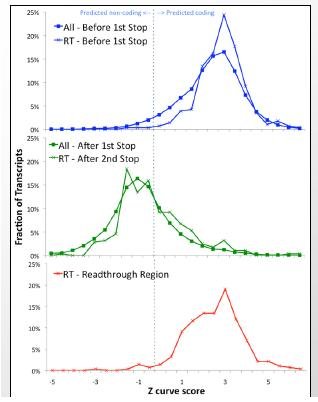
Read–through regions can be determined in a single species based on their pattern of codon usage. The Z–curve as shown in Figure 4.23 measures codon usage patterns in a region of DNA. From the figure, one can observe that the read–through region matches the distribution before the regular stop codon. After the second stop however, the region matches regions found after regular stops.

Another suggestion offered in class was the possibility of ribosome slippage, where the ribosome skips some bases during translation. This might cause the ribosome to skip past a stop codon. This event occurs in bacterial and viral genomes, which have a greater pressure to keep their genomes small, and therefore can use this slipping technique to read a single transcript in each different reading frame. However, humans and flies are not under such extreme pressure to keep their genomes small. Additionally, we showed above that the excess we observe beyond the stop codon is frame specific to frame 0, suggesting that ribosome slipping is not responsible.

Cells are stochastic in general and most processes tolerate mistakes at low frequencies. The system isn’t perfect and stop codon leaks happen. However, the following evidence suggests that stop codon read–through is not random but instead subject to regulatory control:
- Perfect conservation of read–through stop codons is observed in 93% of cases, which is much higher than the 24% found in background.
- Increased conservation is observed upstream of the read–through stop codon.

Figure 4.22: Various interpretations of stop codon suppression. See text for explanation.

All - Before 1st Stop.png — Figure 4.23: Z–curve for Caki. Note that the codon usage in the read through region is similar to that in the region before the first stop codon.

Stop codon bias is observed. TGAC is the most frequent sequence found at the stop codon in read-through and the least frequent found at normal terminated stop codons. It is known to be a “leaky” stop codon. TAAA is found almost universally only in non–read–through instances.

• Unusually high numbers of GCA repeats observed through read–through stop codons.
• Increased RNA secondary structure is observed following transcription suggesting evolutionarily conserved hairpins.

³Kellis M, Patterson N, Endrizzi M, Birren B, Lander E. S. 2003. Sequencing and comparison of yeast species to identify genes and regulatory elements. Science. 423: 241–254.

⁴Clamp M et al. 2007. Distinguishing protein–coding and noncoding genes in the human genome. PNAS. 104: 19428–19433.