
4.3: Excess Constraint
- Page ID
- 40929

In most regions of the genome where we see conservation across species, we expect there to be at least some amount of synonymous substitution. These are “silent” nucleotide substitutions that modify a codon in such a way that the amino acid it encodes is unchanged. In a 2011 paper2, Lindblad–Toh et al. studied evolutionary constraint in the human genome by doing comparative analysis of 29 mammalian species. They found that among the 29 genomes, the average nucleotide site showed 4.5 substitutions per site.
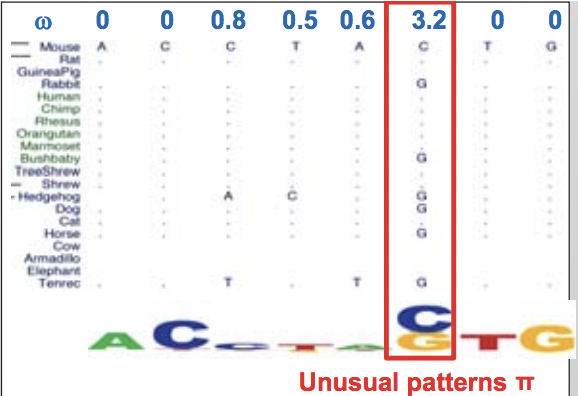
Figure 4.4: This sequence displays an unusual substitution rate of substituting C with G and vice versa.
Given such a high average substitution rate, we do not expect to see perfect conservation across all regions that are conserved. For example, ignoring all other effects, the probability of a 12–mer remaining fixed across all 29 species is less than 10-25. Thus, regions which are nearly perfectly conserved across multiple species stand out as being unique and worthy of further study. One such region is shown in Figure 4.6.
Causes of Excess Constraint
The question is what evolutionary pressures cause certain regions to be so perfectly conserved? The following were all mentioned in class as possibilities:
- Could it be that there is a special structure of DNA shielding this area from mutation?
- Is there some special error correcting machinery that sits at this spot?
- Can the cell use the methylation state of the two copies of DNA as an error correcting mechanism? This mechanism would rely on the fact that the new copy of DNA is unmethylated, and therefore the DNA replication machinery could check the new copy against the old methylated copy.
- Maybe the next generation can’t survive if this region is mutated?
Another possible explanation is that selection is occurring to conserve specific codons. Some codons are more efficient than others: for example, higher abundant proteins that need rapid translation might select codons that give the most efficient translation rate, while other proteins might select for codons that give less efficient translation.
Still, these regions seem too perfectly conserved to be explained by codon usage alone. What else can explain excess constraint? There must be some degree of accuracy needed at the nucleotide level that keeps these sequences from diverging.
It could be that we are looking at the same region in two species that have only recently diverged or that there is a specific genetic mechanism protecting this area. However, it is more likely that so much conservation is a sign of protein coding regions that simultaneously encode other functional elements. For example, the HOXB5 gene shows obvious excess constraint, and there is evidence that the 5’ end of the HOXB5 ORF encodes both protein and an RNA secondary structure.

Figure 4.5: By increasing the number of mammals studied, we see an increase in the constrained k-mers and base pairs that are detectable.
Regions that encode more than one type of functional element are under overlapping selective pressures. There might be pressure in the protein coding space to keep the amino acid sequence corresponding to this region the same, combined with pressure from the RNA space to keep a nucleotide sequence that preserves the RNA’s secondary structure. As a result of these two pressures to keep codons for the same amino acids and to produce the same RNA structure, the region is likely to show much less tolerance for any synonymous substitution patterns.
The process of estimating evolutionary constraint from genomic alignment data across multiple species follows the steps below:
- Count the number of edit operations (i.e. the number of substitutions and/or deletions/insertions)
- Estimate the number of mutations including back-mutations
- Incorporate information about the neighborhood elements of the conserved element by looking at ”conservation windows”
- Estimate the probability of a constrained “hidden state” through using Hidden Markov Models
- Use phylogeny to estimate tree mutation rate (i.e. reject substitutions that should occur along the
tree)
- Allow different portions of the tree to have different mutation rates
Modeling Excess Constraint
To better study region of excess constraint, we develop mathematical models to systematically measure the amount of synonymous and non-synonymous conservation of different regions. We will measure two rates: codon and nucleotide conservation.
To represent the null model, we can build rate matrices (4 × 4 in the nucleotide case and 64 × 64 for the codon case) that give the rates of substitutions between either codons or nucleotides for a unit time. We estimate the rates in the null model by looking at a ton of data and estimating the probabilities of each type of substitution. See Figure 4.18a in 4.5.2 for an example of a null matrix for the codon case.
• λs: the rate of synonymous substitutions

Figure 4.6: Many genomic regions, such as HOXB5, show more conservation than we would expect in normal conserved coding regions. Among the 29 species under study, all but 7 of them had the exact same nucleotide sequence. The green areas are areas that have undergone evolutionary mutations.

Figure 4.7: We can model mutations using rate matrices, as shown here for nucleotide substitutions on the left and codon substitutions on the right. In each matrix, the cell in the mth row and nth column represents the likelihood that the mth symbol will mutate into the nth symbol. The darker the color, the less likely the mutation.
For example, if λs = 0.5, then the rate of synonymous substitutions is half of what is expected from the null model in that region. We can then evaluate the statistical significance of the rate estimates we obtain, and find regions where the rate of substitution is much lower than expected.
Using a null model here helps us account for biases in alignment coverage of certain codons and also accounts for the possibility of codon degeneracy, in which case we would expect to see a much higher rate of substitutions. We will learn how to combine such models with phylogenic methods when we talk about phylogenic trees and evolution later on in the course.
Applying this model shows that the sequences in the first translated codons, cassette exons (exons that are present in one mRNA transcript but absent in an isoform of the transcript), and alternatively spliced regions have especially low rates of synonymous substitutions.
Excess Constraint in the Human Genome
In this section, we will examine the problem of determining the total proportion of the human genome under excess constraint. In particular, we will revisit the work of Lindblad–Toh et al. (2011), which compared 29 mammalian genomes. They measured conservation levels throughout the genome by applying the process described in the previous section to 50–mers. By considering only 50–mers which were part of ancestral repeats, it is possible to determine a background level of conservation. We can imagine that the intensities of conservation among the 50–mers are distributed according to a hidden probability distribution, as illustrated in Figure 4.8. In the figure, the background curve represents the distribution of constraint in the absence of special mechanisms for excess constraint, as determined by looking at ancestral repeats, while the signal (foreground) curve represents the actual distribution of the genome. The signal curve has more conservation overall due to the purifying effects of natural selection.
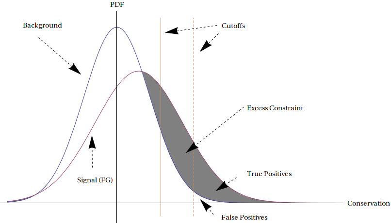
Figure 4.8: Measuring genome–wide excess constraint. See accompanying text for explanation.
We may wish to investigate specific regions of the genome which are under excess constraint by setting a threshold level of conservation and examining regions which are more conserved. In the illustration, this corresponds to considering all 50–mers which fall to the right of one of the orange lines. We see that while this method does indeed give us regions under excess constraint, it also gives us false positives. This is because even in the absence of purifying selection and other effects, certain regions will be heavily conserved, simply due to random chance. Setting the threshold higher, such as by using the dotted orange line as our threshold, reduces the proportion of false positives (FP) to true positives (TP), while also lowering the number of true positives detected, thus trading higher specificity for lower sensitivity.
However, not all hope is lost. It is possible to empirically measure both the background (BG) and foreground (FG) signal curves, as described above. Once that is done, the area of the region between them, which is shaded in gray in Figure 4.8, can be determined by integration. This area represents the proportion of the genome which is under excess constraint. Because the curves overlap, we cannot detect all conserved elements but we can estimate the total amount of excess constraint. This number of estimated constraint turns out to be about 5% of the human genome, depending on how large a window is used. Those regions are likely to all be functional, but since about 1.5% of the human genome is protein–coding, we can infer that the remaining 3.5% consists of functional, non–coding elements, most of which probably play regulatory roles.
We have seen that evolutionary constraint over the whole genome can be estimated by evaluating genomic constraint against a background distribution. Lindblad-Toh et al. (2011) compare genome conservation across 29 mammals against a background calculated from ancestral repeat elements to find regions with excess constraint (Figure 4.9A and B). Annotation of evolutionarily constrained bases reveals that the majority of discovered regions are intergenic and intronic and demonstrates that going from four (HMRD) to 29 mammalian genomes increases the power of this analysis primarily in non-coding regions (Figure 4.9C). The most constrained regions in the genome are coding regions (Figure 4.9D).
As shown in Figure 4.9, the increase from HMRD to a 29 genome alignment vastly improves the power

Figure 4.9: Detecting functional elements from their evolutionary signature. A Distribution of constraint for the whole genome against ancestral repeats (background). B Difference between whole genome and background constraint. C Discovery of functional elements from excess constraint. Novel elements are shown in red. D Enrichment of elements for regions of excess constraint.
of this analysis. However, while the amount of intergenic elements detected increased significantly, detection is still limited by the fact that non-functional elements have much lower species coverage depth in multiple alignments than functional regions (Figure 4.10). For example, ancestral repeats (AR, μ = 11.4) have a much lower average coverage depth than exons (μ = 20.9). On one hand, this shows evidence of selection against insertions and deletions in functional elements, which are not examined in the analysis of base constraint. On the other, it also complicates the analysis of evolutionary constraint, as such work must then handle varying coverage across the genome.
Examples of Excess Constraint
Examples of excess constraint have been found in the following cases:
- Most Hox genes show overlapping constraint regions. In particular, as mentioned above the first 50 amino acids of HOXB5 are almost completely conserved. In addition, HOXA2 shows overlapping regulatory modules. These two loci encode developmental enhancers, providing a mechanism for tissue specific expression.
- ADAR: the main regulator of mRNA editing, has a splice variant where a low synonymous substitution rate was found at a resolution of 9 codons.
- BRCA1: Hurst and Pal (2001) found a low rate of synonymous substitutions in certain regions of BRCA1, the main gene involved in breast cancer. They hypothesized that purifying selection is occur- ring in these regions. (This claim was refuted by Schmid and Yang (2008) who claim this phenomenon is the artifact of a sliding window analysis).
- THRA/NR1D1: these genes, also involved in breast cancer, are part of a dual coding region that codes for both genes and is highly conserved.

Figure 4.10: Coverage depth across different sets of elements.
- SEPHS2: has a hairpin involved in selenocysteine recoding. Because this region must select codons to both conserve the protein’s amino acid sequence and the nucleotides to keep the same RNA secondary structure, it shows excess constraint.
Measuring constraint at individual nucleotides
By measuring evolutionary constraint at individual nucleotides instead of blocks of the sequence, we may find individual transcription factor binding sites, position-specific bias within motif instances, and reveal motif consensus among most species. Specifically, we can detect SNPs that disrupt conserved regulatory motifs and determine the level of evolution by looking at every nucleotide in the gene. By looking at nucleotides individually, we can find SNPs that are important in the function of a specific sequence.
2 www.nature.com/nature/journal...ture10530.html