Biology LibreTexts

2.5: Measuring Height on Irregular Trees

  • Page ID
    20251
  • \( \newcommand{\vecs}[1]{\overset { \scriptstyle \rightharpoonup} {\mathbf{#1}} } \)

    \( \newcommand{\vecd}[1]{\overset{-\!-\!\rightharpoonup}{\vphantom{a}\smash {#1}}} \)

    \( \newcommand{\id}{\mathrm{id}}\) \( \newcommand{\Span}{\mathrm{span}}\)

    ( \newcommand{\kernel}{\mathrm{null}\,}\) \( \newcommand{\range}{\mathrm{range}\,}\)

    \( \newcommand{\RealPart}{\mathrm{Re}}\) \( \newcommand{\ImaginaryPart}{\mathrm{Im}}\)

    \( \newcommand{\Argument}{\mathrm{Arg}}\) \( \newcommand{\norm}[1]{\| #1 \|}\)

    \( \newcommand{\inner}[2]{\langle #1, #2 \rangle}\)

    \( \newcommand{\Span}{\mathrm{span}}\)

    \( \newcommand{\id}{\mathrm{id}}\)

    \( \newcommand{\Span}{\mathrm{span}}\)

    \( \newcommand{\kernel}{\mathrm{null}\,}\)

    \( \newcommand{\range}{\mathrm{range}\,}\)

    \( \newcommand{\RealPart}{\mathrm{Re}}\)

    \( \newcommand{\ImaginaryPart}{\mathrm{Im}}\)

    \( \newcommand{\Argument}{\mathrm{Arg}}\)

    \( \newcommand{\norm}[1]{\| #1 \|}\)

    \( \newcommand{\inner}[2]{\langle #1, #2 \rangle}\)

    \( \newcommand{\Span}{\mathrm{span}}\) \( \newcommand{\AA}{\unicode[.8,0]{x212B}}\)

    \( \newcommand{\vectorA}[1]{\vec{#1}}      % arrow\)

    \( \newcommand{\vectorAt}[1]{\vec{\text{#1}}}      % arrow\)

    \( \newcommand{\vectorB}[1]{\overset { \scriptstyle \rightharpoonup} {\mathbf{#1}} } \)

    \( \newcommand{\vectorC}[1]{\textbf{#1}} \)

    \( \newcommand{\vectorD}[1]{\overrightarrow{#1}} \)

    \( \newcommand{\vectorDt}[1]{\overrightarrow{\text{#1}}} \)

    \( \newcommand{\vectE}[1]{\overset{-\!-\!\rightharpoonup}{\vphantom{a}\smash{\mathbf {#1}}}} \)

    \( \newcommand{\vecs}[1]{\overset { \scriptstyle \rightharpoonup} {\mathbf{#1}} } \)

    \( \newcommand{\vecd}[1]{\overset{-\!-\!\rightharpoonup}{\vphantom{a}\smash {#1}}} \)

    \(\newcommand{\avec}{\mathbf a}\) \(\newcommand{\bvec}{\mathbf b}\) \(\newcommand{\cvec}{\mathbf c}\) \(\newcommand{\dvec}{\mathbf d}\) \(\newcommand{\dtil}{\widetilde{\mathbf d}}\) \(\newcommand{\evec}{\mathbf e}\) \(\newcommand{\fvec}{\mathbf f}\) \(\newcommand{\nvec}{\mathbf n}\) \(\newcommand{\pvec}{\mathbf p}\) \(\newcommand{\qvec}{\mathbf q}\) \(\newcommand{\svec}{\mathbf s}\) \(\newcommand{\tvec}{\mathbf t}\) \(\newcommand{\uvec}{\mathbf u}\) \(\newcommand{\vvec}{\mathbf v}\) \(\newcommand{\wvec}{\mathbf w}\) \(\newcommand{\xvec}{\mathbf x}\) \(\newcommand{\yvec}{\mathbf y}\) \(\newcommand{\zvec}{\mathbf z}\) \(\newcommand{\rvec}{\mathbf r}\) \(\newcommand{\mvec}{\mathbf m}\) \(\newcommand{\zerovec}{\mathbf 0}\) \(\newcommand{\onevec}{\mathbf 1}\) \(\newcommand{\real}{\mathbb R}\) \(\newcommand{\twovec}[2]{\left[\begin{array}{r}#1 \\ #2 \end{array}\right]}\) \(\newcommand{\ctwovec}[2]{\left[\begin{array}{c}#1 \\ #2 \end{array}\right]}\) \(\newcommand{\threevec}[3]{\left[\begin{array}{r}#1 \\ #2 \\ #3 \end{array}\right]}\) \(\newcommand{\cthreevec}[3]{\left[\begin{array}{c}#1 \\ #2 \\ #3 \end{array}\right]}\) \(\newcommand{\fourvec}[4]{\left[\begin{array}{r}#1 \\ #2 \\ #3 \\ #4 \end{array}\right]}\) \(\newcommand{\cfourvec}[4]{\left[\begin{array}{c}#1 \\ #2 \\ #3 \\ #4 \end{array}\right]}\) \(\newcommand{\fivevec}[5]{\left[\begin{array}{r}#1 \\ #2 \\ #3 \\ #4 \\ #5 \\ \end{array}\right]}\) \(\newcommand{\cfivevec}[5]{\left[\begin{array}{c}#1 \\ #2 \\ #3 \\ #4 \\ #5 \\ \end{array}\right]}\) \(\newcommand{\mattwo}[4]{\left[\begin{array}{rr}#1 \amp #2 \\ #3 \amp #4 \\ \end{array}\right]}\) \(\newcommand{\laspan}[1]{\text{Span}\{#1\}}\) \(\newcommand{\bcal}{\cal B}\) \(\newcommand{\ccal}{\cal C}\) \(\newcommand{\scal}{\cal S}\) \(\newcommand{\wcal}{\cal W}\) \(\newcommand{\ecal}{\cal E}\) \(\newcommand{\coords}[2]{\left\{#1\right\}_{#2}}\) \(\newcommand{\gray}[1]{\color{gray}{#1}}\) \(\newcommand{\lgray}[1]{\color{lightgray}{#1}}\) \(\newcommand{\rank}{\operatorname{rank}}\) \(\newcommand{\row}{\text{Row}}\) \(\newcommand{\col}{\text{Col}}\) \(\renewcommand{\row}{\text{Row}}\) \(\newcommand{\nul}{\text{Nul}}\) \(\newcommand{\var}{\text{Var}}\) \(\newcommand{\corr}{\text{corr}}\) \(\newcommand{\len}[1]{\left|#1\right|}\) \(\newcommand{\bbar}{\overline{\bvec}}\) \(\newcommand{\bhat}{\widehat{\bvec}}\) \(\newcommand{\bperp}{\bvec^\perp}\) \(\newcommand{\xhat}{\widehat{\xvec}}\) \(\newcommand{\vhat}{\widehat{\vvec}}\) \(\newcommand{\uhat}{\widehat{\uvec}}\) \(\newcommand{\what}{\widehat{\wvec}}\) \(\newcommand{\Sighat}{\widehat{\Sigma}}\) \(\newcommand{\lt}{<}\) \(\newcommand{\gt}{>}\) \(\newcommand{\amp}{&}\) \(\definecolor{fillinmathshade}{gray}{0.9}\)

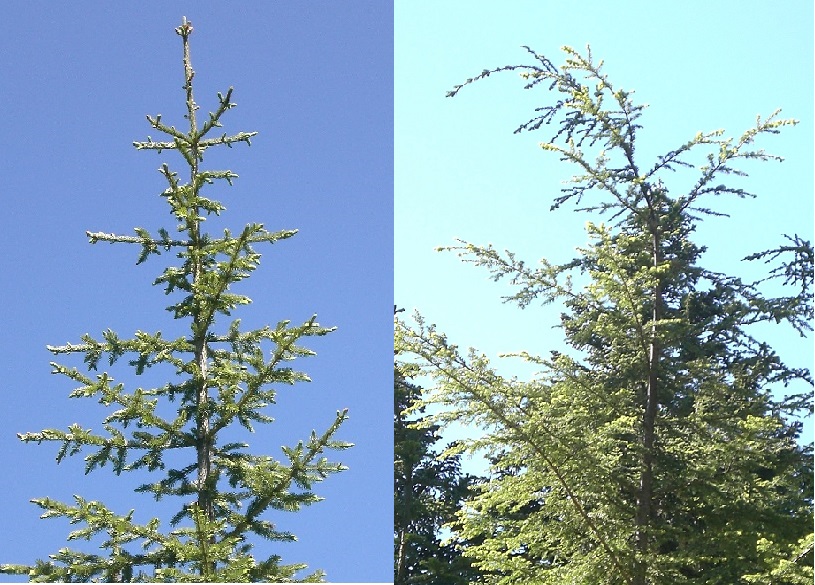
    Species considerations: It is quite easy to measure tree height on conifers because conifers have a very distinct top. Each year’s whorl of growth produces a clear tip with short lateral branches, even on hemlocks (Tsuga spp.)(Figure 2.8).
    conifertops.jpg

    Figure 2.8. Conifers have clear, distinctive tops that make finding the top easy.
    QUKEtop-271x300.png

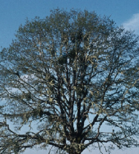
    Figure 2.9. Hardwoods such as this oak (Quercus kelloggii) have rounded or uneven crowns that can make finding the top a little more difficult.

    Hardwoods on the other hand, have rounded crowns that are often a function of the amount of sun they are able to capture (Figure 2.9). Under shaded conditions, they may be very one-sided. On hardwoods, it is extremely important to get a clear view of the whole crown, so that side branches are not mistaken as the top.

    Broken tops

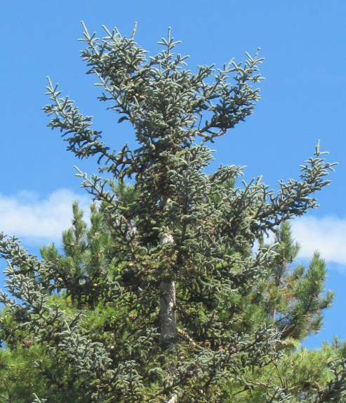
    Trees in which the top has blown out can be tricky. The short or nonexistent tip is often hidden by long lateral branches near the top of the tree. If the top cannot be seen clearly, it is easy to mistake the tips of the lateral branches for the top. A rounded or flat top in a conifer suggests a missing top, and this type of tree should always be examined closely (Figure 2.10). As we saw in Figure 2.6, measuring a lateral branch instead of the tip can overestimate the tree’s height. The closer one is to the tree, the greater the error. This is another reason why it is important to walk a distance far enough from the tree to get a clear view of the top.
    broken4.png

    Figure 2.10. A flat-topped fir tree. When conifers have such “eagle nest” tops, it indicates that the main stem has broken out of the tree. Note how large the diameter is at this point.

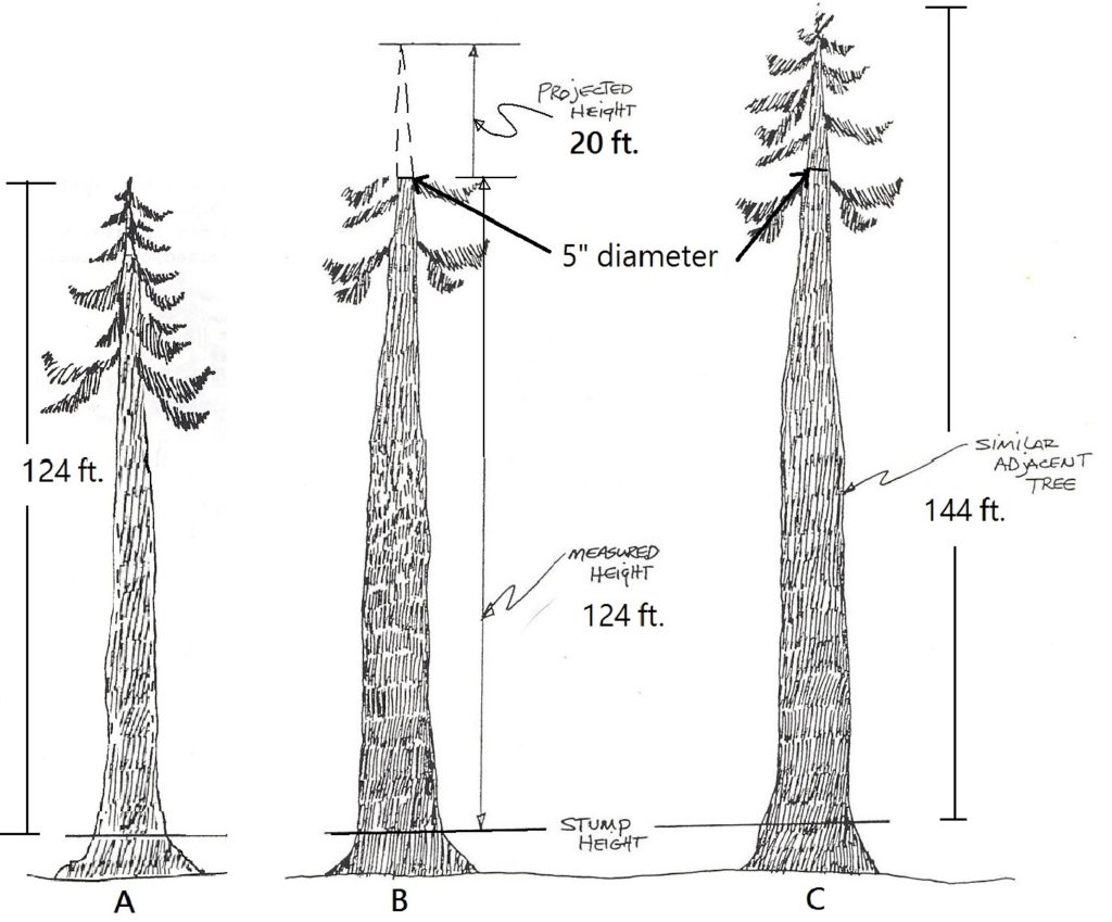
    When measuring total height on trees with broken tops, the tree top must be “reconstructed,” in order to maintain the tree’s correct taper, or “original” shape. Incorrect taper will affect wood volume estimates. A normal tree that is 124’ tall (A below) has a very different shape than a tree whose top has broken out at 124’ (B below). The standard method for reconstructing a tree’s top is to look at the surrounding trees and estimate the broken tree’s missing height from their growth. Let’s say a tree similar in diameter and taper to the broken-top tree below (C below), runs 20 feet from a diameter of five inches to its tip (Figure 2.11). Using this as a guide, one could add 20 feet to the broken-top tree for a reconstructed total height of 144 feet.
    broken-top2-1024x849.jpg

    Figure 2.11. To estimate how much height to add on to a broken-top tree, a neighboring tree that is similar in size and taper is measured and used as a guide. In this example, the top broke out at a diameter of 5 inches. A similar tree was measured from a diameter of 5 inches to its top. This length was 20 feet. Therefore, 20 feet was added to “reconstruct” the top of the broken tree for a total height of 144 feet . (Adapted from [FS] 1990.)

    Leaning trees

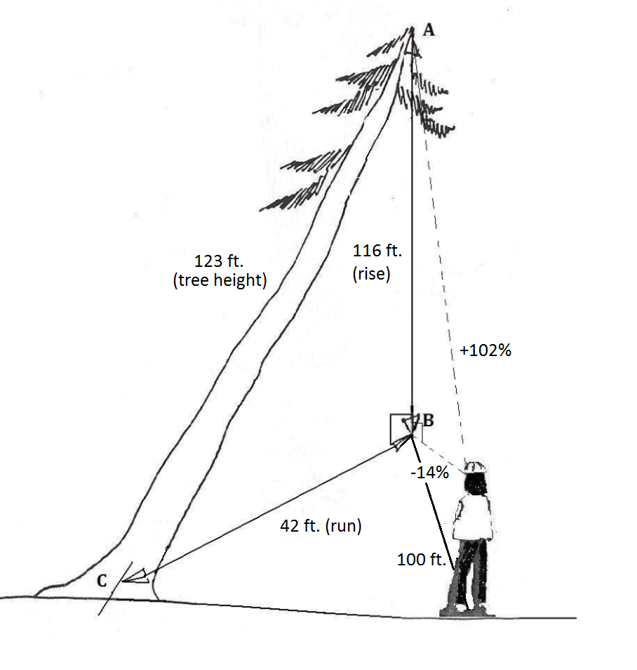
    For a leaning tree, we have to adjust our image of the tree-to-ground triangle. In this case, the leaning tree is the hypotenuse of the triangle instead of the rise (Figure 2.12). The height of the tree can be estimated using the Pythagorean Theorem and the following steps:

    1. Measure out a horizontal distance from the tip of the tree until it is clearly in view.
    2. Calculate the perpendicular distance from the tip of the tree to the ground (rise), using %slope readings as before.
    3. Measure the horizontal distance from the perpendicular drop to the base of the tree (the run).
    4. Once these two sides of the triangle have been determined, estimate the total tree height using the Pythagorean Theorem to solve for the hypotenuse.

    See the example in Figure 2.12 below:
    Leaner1.png

    Figure 2.12. Total height of a leaner tree is determined. (Drawing adapted from [FS] 1990.)

    1. The technician walks out a horizontal distance from fall line AB (in this case 100 ft.).

    2. A %slope reading is taken to the tip of the tree (A, +102%), and then to the point on the ground where the AB fall line intersects the ground (B, (-14%). Using the two %slope readings, the rise of the triangle is determined; in this case, 116 feet.

    3. The horizontal distance between Point B and the stump of the tree (C) is measured with a tape to determine the run; in this case 42 feet.

    4. Finally, using the Pythagorean Theorem, the hypotenuse or height of the tree can be determined.

    55cc0beaef5f5ee2970f310438e8dee6.png

    or

    746c95386559f9072050371b2bcdb9cb.png

    so

    1ab5a6c24b9f524a2a23d8fe2a86f9a4.png

    and

    a6387e2106e571a9e6bc1ed42476128b.png

    c = 123 feet.

    height-fork.jpg

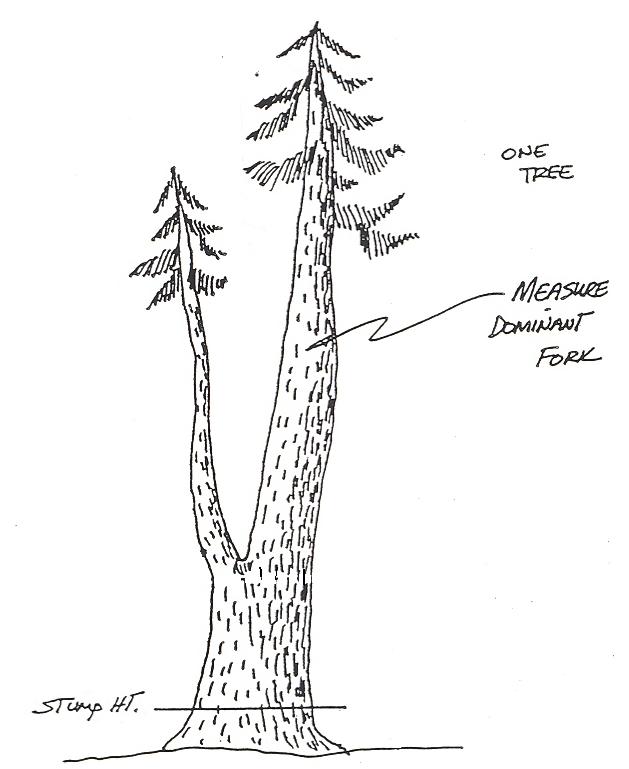
    Figure 2.13. On forked trees, total height is measured from the tree stump to the tip of the tallest fork. (From [FS] 1990.)

    Forked Trees

    On forked trees, the tallest, or dominant fork is measured (Figure 2.13). In some cases, the second fork occurs low enough in the tree to be counted as a second tree, but for most trees, the tallest fork is the only merchantable fork.


    This page titled 2.5: Measuring Height on Irregular Trees is shared under a CC BY license and was authored, remixed, and/or curated by Joan DeYoung (OpenOregon) .

    • Was this article helpful?