
13: Flow Cytometry
- Page ID
- 135774

\( \newcommand{\vecs}[1]{\overset { \scriptstyle \rightharpoonup} {\mathbf{#1}} } \)
\( \newcommand{\vecd}[1]{\overset{-\!-\!\rightharpoonup}{\vphantom{a}\smash {#1}}} \)
\( \newcommand{\dsum}{\displaystyle\sum\limits} \)
\( \newcommand{\dint}{\displaystyle\int\limits} \)
\( \newcommand{\dlim}{\displaystyle\lim\limits} \)
\( \newcommand{\id}{\mathrm{id}}\) \( \newcommand{\Span}{\mathrm{span}}\)
( \newcommand{\kernel}{\mathrm{null}\,}\) \( \newcommand{\range}{\mathrm{range}\,}\)
\( \newcommand{\RealPart}{\mathrm{Re}}\) \( \newcommand{\ImaginaryPart}{\mathrm{Im}}\)
\( \newcommand{\Argument}{\mathrm{Arg}}\) \( \newcommand{\norm}[1]{\| #1 \|}\)
\( \newcommand{\inner}[2]{\langle #1, #2 \rangle}\)
\( \newcommand{\Span}{\mathrm{span}}\)
\( \newcommand{\id}{\mathrm{id}}\)
\( \newcommand{\Span}{\mathrm{span}}\)
\( \newcommand{\kernel}{\mathrm{null}\,}\)
\( \newcommand{\range}{\mathrm{range}\,}\)
\( \newcommand{\RealPart}{\mathrm{Re}}\)
\( \newcommand{\ImaginaryPart}{\mathrm{Im}}\)
\( \newcommand{\Argument}{\mathrm{Arg}}\)
\( \newcommand{\norm}[1]{\| #1 \|}\)
\( \newcommand{\inner}[2]{\langle #1, #2 \rangle}\)
\( \newcommand{\Span}{\mathrm{span}}\) \( \newcommand{\AA}{\unicode[.8,0]{x212B}}\)
\( \newcommand{\vectorA}[1]{\vec{#1}} % arrow\)
\( \newcommand{\vectorAt}[1]{\vec{\text{#1}}} % arrow\)
\( \newcommand{\vectorB}[1]{\overset { \scriptstyle \rightharpoonup} {\mathbf{#1}} } \)
\( \newcommand{\vectorC}[1]{\textbf{#1}} \)
\( \newcommand{\vectorD}[1]{\overrightarrow{#1}} \)
\( \newcommand{\vectorDt}[1]{\overrightarrow{\text{#1}}} \)
\( \newcommand{\vectE}[1]{\overset{-\!-\!\rightharpoonup}{\vphantom{a}\smash{\mathbf {#1}}}} \)
\( \newcommand{\vecs}[1]{\overset { \scriptstyle \rightharpoonup} {\mathbf{#1}} } \)
\(\newcommand{\longvect}{\overrightarrow}\)
\( \newcommand{\vecd}[1]{\overset{-\!-\!\rightharpoonup}{\vphantom{a}\smash {#1}}} \)
\(\newcommand{\avec}{\mathbf a}\) \(\newcommand{\bvec}{\mathbf b}\) \(\newcommand{\cvec}{\mathbf c}\) \(\newcommand{\dvec}{\mathbf d}\) \(\newcommand{\dtil}{\widetilde{\mathbf d}}\) \(\newcommand{\evec}{\mathbf e}\) \(\newcommand{\fvec}{\mathbf f}\) \(\newcommand{\nvec}{\mathbf n}\) \(\newcommand{\pvec}{\mathbf p}\) \(\newcommand{\qvec}{\mathbf q}\) \(\newcommand{\svec}{\mathbf s}\) \(\newcommand{\tvec}{\mathbf t}\) \(\newcommand{\uvec}{\mathbf u}\) \(\newcommand{\vvec}{\mathbf v}\) \(\newcommand{\wvec}{\mathbf w}\) \(\newcommand{\xvec}{\mathbf x}\) \(\newcommand{\yvec}{\mathbf y}\) \(\newcommand{\zvec}{\mathbf z}\) \(\newcommand{\rvec}{\mathbf r}\) \(\newcommand{\mvec}{\mathbf m}\) \(\newcommand{\zerovec}{\mathbf 0}\) \(\newcommand{\onevec}{\mathbf 1}\) \(\newcommand{\real}{\mathbb R}\) \(\newcommand{\twovec}[2]{\left[\begin{array}{r}#1 \\ #2 \end{array}\right]}\) \(\newcommand{\ctwovec}[2]{\left[\begin{array}{c}#1 \\ #2 \end{array}\right]}\) \(\newcommand{\threevec}[3]{\left[\begin{array}{r}#1 \\ #2 \\ #3 \end{array}\right]}\) \(\newcommand{\cthreevec}[3]{\left[\begin{array}{c}#1 \\ #2 \\ #3 \end{array}\right]}\) \(\newcommand{\fourvec}[4]{\left[\begin{array}{r}#1 \\ #2 \\ #3 \\ #4 \end{array}\right]}\) \(\newcommand{\cfourvec}[4]{\left[\begin{array}{c}#1 \\ #2 \\ #3 \\ #4 \end{array}\right]}\) \(\newcommand{\fivevec}[5]{\left[\begin{array}{r}#1 \\ #2 \\ #3 \\ #4 \\ #5 \\ \end{array}\right]}\) \(\newcommand{\cfivevec}[5]{\left[\begin{array}{c}#1 \\ #2 \\ #3 \\ #4 \\ #5 \\ \end{array}\right]}\) \(\newcommand{\mattwo}[4]{\left[\begin{array}{rr}#1 \amp #2 \\ #3 \amp #4 \\ \end{array}\right]}\) \(\newcommand{\laspan}[1]{\text{Span}\{#1\}}\) \(\newcommand{\bcal}{\cal B}\) \(\newcommand{\ccal}{\cal C}\) \(\newcommand{\scal}{\cal S}\) \(\newcommand{\wcal}{\cal W}\) \(\newcommand{\ecal}{\cal E}\) \(\newcommand{\coords}[2]{\left\{#1\right\}_{#2}}\) \(\newcommand{\gray}[1]{\color{gray}{#1}}\) \(\newcommand{\lgray}[1]{\color{lightgray}{#1}}\) \(\newcommand{\rank}{\operatorname{rank}}\) \(\newcommand{\row}{\text{Row}}\) \(\newcommand{\col}{\text{Col}}\) \(\renewcommand{\row}{\text{Row}}\) \(\newcommand{\nul}{\text{Nul}}\) \(\newcommand{\var}{\text{Var}}\) \(\newcommand{\corr}{\text{corr}}\) \(\newcommand{\len}[1]{\left|#1\right|}\) \(\newcommand{\bbar}{\overline{\bvec}}\) \(\newcommand{\bhat}{\widehat{\bvec}}\) \(\newcommand{\bperp}{\bvec^\perp}\) \(\newcommand{\xhat}{\widehat{\xvec}}\) \(\newcommand{\vhat}{\widehat{\vvec}}\) \(\newcommand{\uhat}{\widehat{\uvec}}\) \(\newcommand{\what}{\widehat{\wvec}}\) \(\newcommand{\Sighat}{\widehat{\Sigma}}\) \(\newcommand{\lt}{<}\) \(\newcommand{\gt}{>}\) \(\newcommand{\amp}{&}\) \(\definecolor{fillinmathshade}{gray}{0.9}\)Summary
Flow cytometry is a biotechnology that can be used for many applications. This entry focuses on its use to detect the level of biomarkers present on individual cells in a sample.
Also known as:
Fluorescence-activated cell sorting, FACS
Technically speaking, FACS is a derivative of flow cytometry that physically separates cells into different populations based on their characteristics. By flow cytometry it’s also possible to simply observe those different characteristics without separating the cells.
Samples needed
Single-cell suspension.
Cells will be treated in different ways depending on the measurement being made. Often, cells are immunostained for cell-surface biomarkers (i.e. proteins). Flow cytometry can be used with immunostaining for intracellular biomarkers if they are first fixed and then permeabilized to allow the antibody to enter the cells.
Method
Here, we are describing the use of flow cytometry to detect cell-surface proteins. The cells are first separated to form a single-cell suspension in an appropriate buffer. Then they are immunostained for one or several cell-surface markers. The number of cell surface markers that can be detected in one experiment is limited only by the number of different wavelengths of light that can be simultaneously detected and resolved by the particular flow cytometer being used.

The cells are then allowed to pass through the flow cytometer one at a time. For each cell, two parameters called forward scatter (FSC) and side scatter (SSC) are measured, which give information about cell size and internal complexity (i.e. “granularity”), respectively. The intensity of each fluorescence signal is also measured to determine how much of each biomarker is present on the cell surface.
Controls
Recommended controls are numerous and beyond the scope of this Encyclopedia. However, they are rarely shown in published studies unless the study specifically aims to develop a new method.
Interpretation
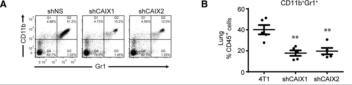
In this experiment, the study authors have established orthotopic tumors in mice using 4T1 mouse breast cancer cells. The 4T1 cells express either a control shRNA (shNS), or one of two shRNAs against CAIX. The authors want to know how the level of CAIX expression in the tumor affects the presence in the mouse lungs of a certain subset of cells that highly express the proteins CD11b and Gr1 on their surface. To do this, the authors removed the lungs from the mice and processed them to a single-cell suspension. The cells were then immunostained for CD45, CD11b, and Gr1. CD45 is a general leukocyte marker, and Panels A and B are only showing cells from the lung that have high CD45 staining; CD45 low cells are excluded from the analysis. In the scatterplots in Panel A, each point on the graph is a cell, positioned based on the intensity of the CD11b and Gr1 staining. The researchers have divided the plot into quadrants that show the cells as “low” or “high” for each of the two biomarkers. Panel B is a dot plot that quantifies the results from Panel A by showing the overall % of the CD45+ cells in each sample that are CD11b+Gr1+. Based on this data, the authors conclude that when the primary tumor does not express CAIX, fewer CD11b+Gr1+ cells are found in the lung.
Image Descriptions
Figure 1 image description:
Single cells passing through a funnel-shaped structure in a flow cytometer. Cells are either red to show the presence of the cell surface protein or black to show its absence. As the cells pass through the narrow part of the “funnel,” they are hit by a laser, and scattered light is detected by one of two detectors, one for forward scatter and one for side scatter. As cells come out of the “funnel” in droplets, the droplets are charged, and can be electromagnetically attracted into one of two tubes: one containing only red cells and one containing only black cells. Side panel shows a cartoon of an antibody attached to a red fluorescent dye binding to a cell-surface protein on a cell. ↵
Figure 2 image description:
Panel A shows three scatterplots. The % of cells (points) in each quadrant of the scatterplot are shown in the table below.
|
shNS |
shCAIX1 |
shCAIX2 |
||
|---|---|---|---|---|
|
Percent of cells |
CD11b high, Gr1 low (upper left) |
4.88 |
4.73 |
4.56 |
|
CD11b high, Gr1 high (upper right) |
51.2 |
15.2 |
12.0 |
|
|
CD11b low, Gr1 high (lower right) |
1.22 |
1.45 |
1.20 |
|
|
CD11b low, Gr1 lo2 (lower left) |
42.7 |
78.6 |
82.3 |
Panel B shows a dot plot comparing the % of CD45 positive cells that are CD11b+Gr1+ in the three samples. It is a quantification of the scatterplots in Panel A. The 4T1 sample shows an average of 40%, whereas both of the shCAIX samples show averages around 20%. ↵
Thumbnail
"Flow cytometry histogram.png"↗ by Kwz at Polish Wikipedia is licensed under the GNU Free Documentation License↗, Version 1.2 or any later version published by the Free Software Foundation↗; with no Invariant Sections, no Front-Cover Texts, and no Back-Cover Texts.
Description: Histogram of a blood sample studied with a flow cytometer.
Author
Katherine Mattaini, Tufts University
- Chafe, S. C., Y. Lou, J. Sceneay, M. Vallejo, M. J. Hamilton, P. C. McDonald, K. L. Bennewith, A. Möller, and S. Dedhar. 2015. Carbonic anhydrase IX promotes myeloid-derived suppressor cell mobilization and establishment of a metastatic niche by stimulating G-CSF production. Cancer Research 75:996-1008. ↵