
8: Cox Proportional Hazards Analysis
- Page ID
- 135771

\( \newcommand{\vecs}[1]{\overset { \scriptstyle \rightharpoonup} {\mathbf{#1}} } \)
\( \newcommand{\vecd}[1]{\overset{-\!-\!\rightharpoonup}{\vphantom{a}\smash {#1}}} \)
\( \newcommand{\dsum}{\displaystyle\sum\limits} \)
\( \newcommand{\dint}{\displaystyle\int\limits} \)
\( \newcommand{\dlim}{\displaystyle\lim\limits} \)
\( \newcommand{\id}{\mathrm{id}}\) \( \newcommand{\Span}{\mathrm{span}}\)
( \newcommand{\kernel}{\mathrm{null}\,}\) \( \newcommand{\range}{\mathrm{range}\,}\)
\( \newcommand{\RealPart}{\mathrm{Re}}\) \( \newcommand{\ImaginaryPart}{\mathrm{Im}}\)
\( \newcommand{\Argument}{\mathrm{Arg}}\) \( \newcommand{\norm}[1]{\| #1 \|}\)
\( \newcommand{\inner}[2]{\langle #1, #2 \rangle}\)
\( \newcommand{\Span}{\mathrm{span}}\)
\( \newcommand{\id}{\mathrm{id}}\)
\( \newcommand{\Span}{\mathrm{span}}\)
\( \newcommand{\kernel}{\mathrm{null}\,}\)
\( \newcommand{\range}{\mathrm{range}\,}\)
\( \newcommand{\RealPart}{\mathrm{Re}}\)
\( \newcommand{\ImaginaryPart}{\mathrm{Im}}\)
\( \newcommand{\Argument}{\mathrm{Arg}}\)
\( \newcommand{\norm}[1]{\| #1 \|}\)
\( \newcommand{\inner}[2]{\langle #1, #2 \rangle}\)
\( \newcommand{\Span}{\mathrm{span}}\) \( \newcommand{\AA}{\unicode[.8,0]{x212B}}\)
\( \newcommand{\vectorA}[1]{\vec{#1}} % arrow\)
\( \newcommand{\vectorAt}[1]{\vec{\text{#1}}} % arrow\)
\( \newcommand{\vectorB}[1]{\overset { \scriptstyle \rightharpoonup} {\mathbf{#1}} } \)
\( \newcommand{\vectorC}[1]{\textbf{#1}} \)
\( \newcommand{\vectorD}[1]{\overrightarrow{#1}} \)
\( \newcommand{\vectorDt}[1]{\overrightarrow{\text{#1}}} \)
\( \newcommand{\vectE}[1]{\overset{-\!-\!\rightharpoonup}{\vphantom{a}\smash{\mathbf {#1}}}} \)
\( \newcommand{\vecs}[1]{\overset { \scriptstyle \rightharpoonup} {\mathbf{#1}} } \)
\(\newcommand{\longvect}{\overrightarrow}\)
\( \newcommand{\vecd}[1]{\overset{-\!-\!\rightharpoonup}{\vphantom{a}\smash {#1}}} \)
\(\newcommand{\avec}{\mathbf a}\) \(\newcommand{\bvec}{\mathbf b}\) \(\newcommand{\cvec}{\mathbf c}\) \(\newcommand{\dvec}{\mathbf d}\) \(\newcommand{\dtil}{\widetilde{\mathbf d}}\) \(\newcommand{\evec}{\mathbf e}\) \(\newcommand{\fvec}{\mathbf f}\) \(\newcommand{\nvec}{\mathbf n}\) \(\newcommand{\pvec}{\mathbf p}\) \(\newcommand{\qvec}{\mathbf q}\) \(\newcommand{\svec}{\mathbf s}\) \(\newcommand{\tvec}{\mathbf t}\) \(\newcommand{\uvec}{\mathbf u}\) \(\newcommand{\vvec}{\mathbf v}\) \(\newcommand{\wvec}{\mathbf w}\) \(\newcommand{\xvec}{\mathbf x}\) \(\newcommand{\yvec}{\mathbf y}\) \(\newcommand{\zvec}{\mathbf z}\) \(\newcommand{\rvec}{\mathbf r}\) \(\newcommand{\mvec}{\mathbf m}\) \(\newcommand{\zerovec}{\mathbf 0}\) \(\newcommand{\onevec}{\mathbf 1}\) \(\newcommand{\real}{\mathbb R}\) \(\newcommand{\twovec}[2]{\left[\begin{array}{r}#1 \\ #2 \end{array}\right]}\) \(\newcommand{\ctwovec}[2]{\left[\begin{array}{c}#1 \\ #2 \end{array}\right]}\) \(\newcommand{\threevec}[3]{\left[\begin{array}{r}#1 \\ #2 \\ #3 \end{array}\right]}\) \(\newcommand{\cthreevec}[3]{\left[\begin{array}{c}#1 \\ #2 \\ #3 \end{array}\right]}\) \(\newcommand{\fourvec}[4]{\left[\begin{array}{r}#1 \\ #2 \\ #3 \\ #4 \end{array}\right]}\) \(\newcommand{\cfourvec}[4]{\left[\begin{array}{c}#1 \\ #2 \\ #3 \\ #4 \end{array}\right]}\) \(\newcommand{\fivevec}[5]{\left[\begin{array}{r}#1 \\ #2 \\ #3 \\ #4 \\ #5 \\ \end{array}\right]}\) \(\newcommand{\cfivevec}[5]{\left[\begin{array}{c}#1 \\ #2 \\ #3 \\ #4 \\ #5 \\ \end{array}\right]}\) \(\newcommand{\mattwo}[4]{\left[\begin{array}{rr}#1 \amp #2 \\ #3 \amp #4 \\ \end{array}\right]}\) \(\newcommand{\laspan}[1]{\text{Span}\{#1\}}\) \(\newcommand{\bcal}{\cal B}\) \(\newcommand{\ccal}{\cal C}\) \(\newcommand{\scal}{\cal S}\) \(\newcommand{\wcal}{\cal W}\) \(\newcommand{\ecal}{\cal E}\) \(\newcommand{\coords}[2]{\left\{#1\right\}_{#2}}\) \(\newcommand{\gray}[1]{\color{gray}{#1}}\) \(\newcommand{\lgray}[1]{\color{lightgray}{#1}}\) \(\newcommand{\rank}{\operatorname{rank}}\) \(\newcommand{\row}{\text{Row}}\) \(\newcommand{\col}{\text{Col}}\) \(\renewcommand{\row}{\text{Row}}\) \(\newcommand{\nul}{\text{Nul}}\) \(\newcommand{\var}{\text{Var}}\) \(\newcommand{\corr}{\text{corr}}\) \(\newcommand{\len}[1]{\left|#1\right|}\) \(\newcommand{\bbar}{\overline{\bvec}}\) \(\newcommand{\bhat}{\widehat{\bvec}}\) \(\newcommand{\bperp}{\bvec^\perp}\) \(\newcommand{\xhat}{\widehat{\xvec}}\) \(\newcommand{\vhat}{\widehat{\vvec}}\) \(\newcommand{\uhat}{\widehat{\uvec}}\) \(\newcommand{\what}{\widehat{\wvec}}\) \(\newcommand{\Sighat}{\widehat{\Sigma}}\) \(\newcommand{\lt}{<}\) \(\newcommand{\gt}{>}\) \(\newcommand{\amp}{&}\) \(\definecolor{fillinmathshade}{gray}{0.9}\)Summary
Cox proportional hazards analysis is a type of survival analysis. Generally speaking, a survival analysis is a mathematical method that models a) the length of time until an event occurs and b) whether that event occurs at all as a function of a number of variables of interest.
I am going to write a very basic-level understanding here, since I am not a mathematician, nor are most of the target audience for this Encyclopedia. I found the videos on survival analysis from “MarinStatsLectures-R Programming & Statistics” on Youtube↗ to be really useful. They’re what helped me write this entry rather than just having a vague idea of what was going on.
Also known as:
Cox PH, Cox regression
Samples needed
Dataset with independent variables of interest & time until target event
Method
As stated above, a survival analysis is a mathematical method that models a) whether an event occurs and b) the time it takes to occur as a function of a number of independent variables. So, for instance, you could use a dataset to predict how long a person is likely to survive after a lung cancer diagnosis (here, “event” = death) based on age at diagnosis, tumor stage at diagnosis, assigned sex, smoking history, etc.
Cox PH analysis is one particular type of survival analysis. The goal of Cox PH is to estimate something called a hazard ratio (HR) rather than to predict the length of survival. Let’s use the example of lung cancer above. A hazard ratio tells you how many times more likely a person from one group (i.e. a past or current smoker) is to die of lung cancer than a person another group (i.e. a never-smoker) at a given moment in time.
Not every analysis that uses this kind of math has death as an end point. When you’re looking at a Cox PH analysis, always ask yourself what the “event” or “outcome” is that’s being analyzed.
So, for the lung cancer example above, you could have a dataset something like this:
| Time from diagnosis to evaluation for event (months) | Did the event happen? (i.e. death) | Age at diagnosis | Tumor stage at diagnosis | …..(list all variables) | |
|---|---|---|---|---|---|
| Patient 1 | 7 | Yes → 1 | 68 | IV → 4 | |
| Patient 2 | 50 | No → 0 | 75 | II → 2 | |
| … (list all patients) | |||||
| Dependent variables | Independent variables | ||||
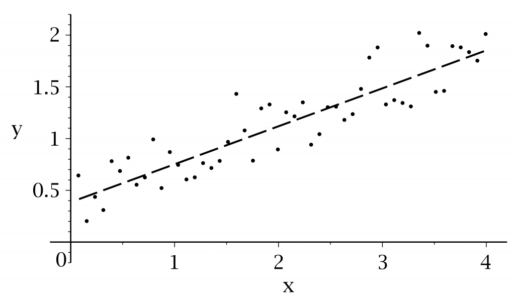
Step 1: Each patient would be a point & you would plot this data. (If you were doing just age vs. survival, it would be plotted in 2D space, if age and tumor stage vs. survival, it would be plotted in 3D space, etc.)
Step 2: Perform regression analysis. This basically means you use a computer program to figure out what constant values make the data points fit a certain equation. For example, you may be familiar with linear regression. The equation of a line is y = mx + b. So, if you plot a bunch of x-y points and use a computer program to find the best fit line, you can get the values of m (slope) & b (intercept). (See Figure 1.)
Cox PH analysis is just like this, except you are fitting a much more complicated equation:
\[Hazard(t) = h_0 (t) + e^{{b_1}{x_1}+{b_2}{x_2}+...}\]
In this equation, the x’s are the independent variables like age at diagnosis, tumor stage at diagnosis, etc. The b’s are the regression coefficients. They determine how important each independent variable is to the outcome.
So, what’s the outcome? Your computer program gives you the b values from the equation above, which can be easily converted into a hazard ratio for each independent variable.
How do you interpret the HR? Say from the example above you found an HR of 1.2 when comparing smokers to non-smokers. That means that for people diagnosed with lung cancer, people who are current or previous smokers are 1.2 times more likely to die from their lung cancer at any given moment in time than those who have lung cancer but never smoked. (Or in other words, they’re 20% more likely to die.) This is “adjusted for” their age at diagnosis, tumor stage at diagnosis, assigned sex, and any other independent variables that were included in the analysis. So, this HR tells you just the effect of their smoking status on survival.
Controls
Beyond the scope of this work!
Thumbnail
"Kaplan-Meier plot of AML survival.svg"↗ by Michaelg2015 is licensed under CC BY-SA 4.0↗.
Description: Kaplan-Meier plot of AML survival for aml data set from R survival package.
Author
Katherine Mattaini, Tufts University
Reviewed by Joshua Abston, Roger Williams University, B.S. Applied Mathematics
Content last updated on April 12, 2022