13.1: Introduction

Cryptozoology

Cryptozoology is a pseudoscience centered around the description of animals that have little or no evidence of existing. These mythical beasts include Bigfoot, Yeti, Sasquatch, jackalope, Loch Ness Monster, and chupacabra. Little evidence exists to illustrate their existence other than folklore.

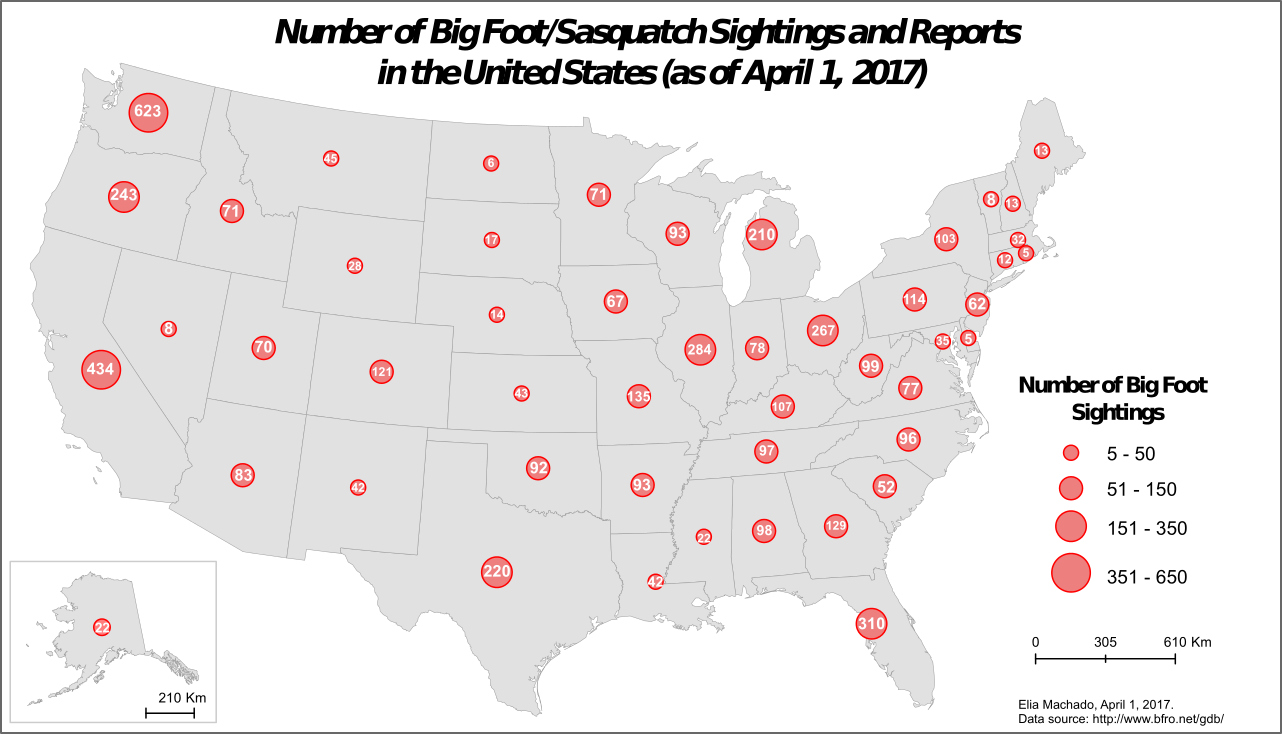
Sightings of Bigfoot in North America. Credit: Elia Machado (CC-BY-NC-SA)

Sometimes, physical evidence is left behind like hair or feces. With DNA evidence, we can help to confirm the existence of these unknown creatures. Below features a table from Sykes et al. displaying results on supposed cryptic Apes (Bigfoot/Yeti) and what DNA evidence has revealed them to be.

Cryptozoological samples of hair believed to arise from legendary animals like Bigfoot, Sasquatch, Yeti, etc.

Table taken from http://rspb.royalsocietypublishing.org/content/281/1789/20140161 CC-BY

The Need for Barcoding

Taxonomy of living things was created by Carl von Linné, who formalized it by using a binomial classification system to differentiate organisms. Binomial nomenclature was used to describe a genus and a species name to each organism to provide an identity. These days, classifications of organisms is becoming increasingly important as a measurement of diversity in the face of habitat destruction and global climate change. There is no consensus on how many life forms exist on this planet, but the estimation of extinction rates is about 1 species per 100-1000 million species. Classification in Linné’s day was mostly performed by morphological differences. This was carried on in fossils. However, morphology has many drawbacks, especially in sexually dimorphic species or species with multiple developmental morphologies.

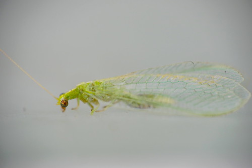
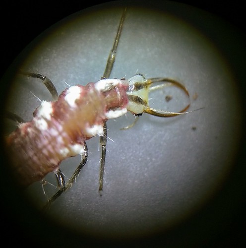
Larva (top) of the Green Lacewing and the adult (bottom)

Molecular biology and DNA technologies have revolutionized the classification system of living things especially in providing the ability to match relatedness of these species. DNA barcoding, like the name implies, seeks to utilize DNA markers to differentially identify organisms. But what DNA markers should be used? What criteria do we use to develop barcodes? Discrimination, Universality, and Robustness are the criteria used to define the usefulness of barcodes.

Since the goal of barcoding is to define specific organisms, discrimination is the primary objective. Discrimination refers to the difference of sequences that occur between species. However, science is easier when there is some universality in the locus used for discrimination. As it sounds, universality is an attempt to use the same locus in disparate genomes. While discrimination is about the uniqueness of sequences, universality seeks to use a single set of PCR primers that will be able to amplify that same distinct region with variable sequence similarity. If some region of DNA has absolutely no sequence deviation between species, this has great universality but poor discrimination. But if a sequence has very low sequence similarity, this is great for discrimination but has absolutely no universality and can not be amplified with the same set of primers. Robustness refers to the reliability of PCR amplification of a region. Some regions of DNA just don’t amplify well or it is too difficult to design appropriate and unique primers for that locus.

A case where there is universality for designing primers, but not an area where discrimination can occur.

While discrimination of different organisms can occur in this situation, the lack of similarity in sequence would make it difficult to design primers. That is, the lack of universality in sequence would also make this PCR not robust.

Enough variability in these sequences gives us the ability to discriminate between species. The high similarity provides us the universality required to design primers that may be robust enough to amplify by PCR.

Sometimes, species are so similar for one sequence that a second marker is required. Just as the standard UPC barcode has a series of vertical lines of different spacing and width, a 2-dimensional barcode adds that second dimension of information into a square of dots like in a QR code (Quick Response code). We can also utilize the second, the third, or the fourth set of loci that will aid in increased discrimination just as CoDIS utilizes multiple STR sites to define individual people. In animals, the most commonly used barcode is the mitochondrial gene, Cytochrome Oxidase I (COI). Since all animals have mitochondria and have this mitochondrial gene, it offers high universality. It is a robust locus that is easy to amplify and has high copy number with enough sequence deviation between species to discriminate between them.

Animal mitochondrial genomes vary from 16kb-22kb. However, plants, fungi, and protists have wildly different and larger mitochondrial genomes. For plants, we use a chloroplast gene, ribulose-bisphosphate carboxylase large subunit (rbcL) or maturase K (matK) (Hollingsworth et al. 2011). Prokaryotes are often discriminated by their 16s rRNA gene while eukaryotes can be identified by 18s rRNA. COI (a maternally transmitted gene) will not create a clear picture of species identity in the case of hybrid animals (mules, ligers, coydogs, etc.). Sometimes, closely related species are also indistinguishable by a single barcode, so the inclusion of 18s with COI may be necessary to define the identity of the species. Since it is so difficult to meet the three criteria (robustness, universality, and discrimination) for all species, having these multiple barcodes is important. Fungi prove to be difficult in identification by COI, so another marker called the internal transcribed spacer (ITS) is used to aid in their identification. We must also remember that not everything with chloroplasts are plants and, therefore, additional markers are used to identify protists.

Mixtures of Organisms

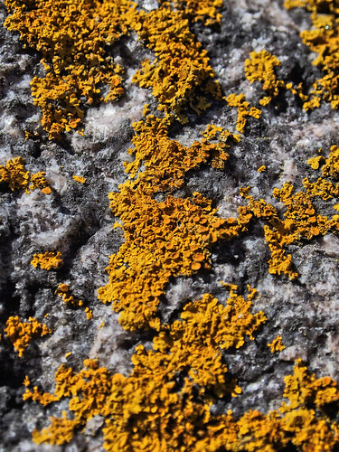
Lichens are composite organisms composed of cyanobacteria or other algae with fungi. In this case, a single barcode would incorrectly identify the species.

Kefir granules represent colonies of mixed microbes that are used to generate kefir. Credit: A. Kniesel (CC-BY-SA 3.0)

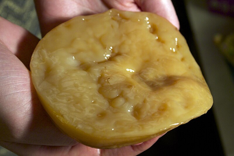
A symbiotic colony of bacteria and yeast is used to ferment kombucha. As the name implies, this is a complex composite colony of multiple species that contribute to the qualities of the kombucha. Credit: Lukas Chin (CC-BY-SA 4.0)

Metabarcoding and Microbiomes

Class Results

Students wanted to check some food items. These included breakfast sausage from a Halal cart, “beef jerky” from the vending machine, roast beef from the cafeteria, and Chinese sausage (lopcheng).

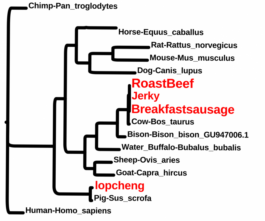
For more class results, please visit https://openlab.citytech.cuny.edu/dna-barcodes/

Further Resources

• Reference Sequences
  • Gorilla COI: FASTA
  • Apple rbcL: FASTA
  • Staphylococcus 16S: FASTA
  • Toxoplasma 18S: FASTA
  • Porcinni mushroom ITS: FASTA
• Sykes BC, Mullis RA, Hagenmuller C, Melton TW, Sartori M. Genetic analysis of hair samples attributed to yeti, bigfoot and other anomalous primates. Proc Biol Sci. 2014 Aug 22;281(1789):20140161. doi: 10.1098/rspb.2014.0161.
• Hollingsworth PM, Graham SW, Little DP (2011) Choosing and Using a Plant DNA Barcode. PLOS ONE 6(5): e19254. https://doi.org/10.1371/journal.pone.0019254
• http://www.dnabarcoding101.org/