12.2: Maternal Lineage

Mitochondrial and Maternal Inheritance

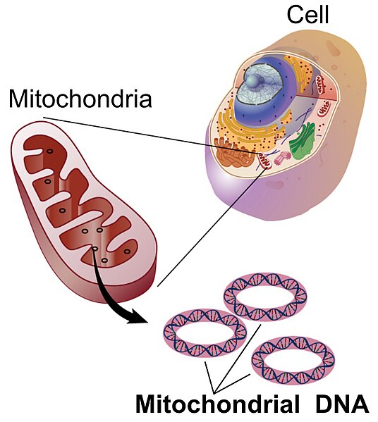
In addition to the 23 chromosomes inherited from mother and 23 chromosomes inherited from father, humans have an additional genome that is only inherited from the mother. This genome comes from the endosymbiotic organelle, the mitochondrion.

Mitochondria are thought to have arisen in the eukaryotic line when bacteria capable of detoxifying the deadly effects of atmospheric oxygen were engulfed by a eukaryote that did not proceed to consume it. Over the course of time, these formerly free-living bacteria became dependent on the eukaryotic cell environment while providing the benefit to the host cell of aerobic respiration. Hallmarks of this endosymbiotic event include the inner prokaryotic membrane surrounded by the outer eukaryotic membrane, the presence of prokaryotic ribosomes and most significantly, and the circular prokaryotic chromosome. Mitochondria still replicate independently of the host cell but can not survive outside of this cellular environment. Animal mitochondria have the simplest genomes of all mitochondrial genomes, ranging from 11-28kb. The human mitochondrial genome consists of 37 genes which are almost all devoted to processing ATP through oxidative phosphorylation.

Human mitochondrial genome

The human mitochondrial genome (genbank file) consists of 16,569 nucleotides (16.6kb). While most of this 16.6kb genome consists of protein-encoding genes, approximately 1.2kb non-coding DNA takes part in signals that control the expression of these genes and replication processes. It is the area of DNA where the double-strandedness is displaced and having the name D-loop (displacement loop). Mutations in this area generally have very little effect on the functioning of the mitochondria. Because of this reduced selection pressure on this area, this control region is also referred to as the hypervariable region. This hypervariable region actually has 10 times more SNPs than the nuclear genome. Due to this abundance of mutations, it is possible to track down the maternal line of an individual. Why just maternal? The human oocyte contains many mitochondria while sperm cells only contain mitochondria that power the flagellar motion. Upon fertilization, the flagellum and the associated mitochondria are lost, leaving the zygote with only maternal mitochondria.

The cluster of SNPs found in the mitochondrial control region are linked and are always inherited together. Because of the lack of paternal contribution, this linkage is referred to as a haplotype, or “half-type”. Tracking these polymorphic haplotypes, a family tree of humans was developed in the 1980s which concluded that humans arose from a metaphorical “Mitochondrial Eve” 200,000 years ago. As a metaphor to the Biblical Eve, this alludes to an origin but unlike the Biblical event, this does not mean that it was a single woman that gave rise to all of modern humanity. On the contrary, the metaphor merely indicates that a series of females; sisters and cousins, of this line gave rise to modern humans.

Migration map of mitochondrial haplogroups. Numbers represent 1000 years ago.

The use of mitochondria for this analysis provides great flexibility, especially from ancient sources. Unlike the nuclear genome which only has 2 copies of DNA per cell, the mitochondria are abundant in number and provide many copies of genome per cell. Ancient sources of DNA in fossils will most often have degradation of the DNA. The mitochondrial genome is just as likely to undergo degradation over time. However, the high copy number allows for gaps to be filled in easily. SNPs do not alter the overall size of the hypervariable region, therefore amplification by PCR can not resolve these differences based on agarose gel migration. However, amplicons (amplified copies) can be sent for sequencing whereby each nucleotide can be called out in succession and reveal the specific SNPs.