9.4: Probability and Chi-Square Analysis
- Page ID
- 24809

\( \newcommand{\vecs}[1]{\overset { \scriptstyle \rightharpoonup} {\mathbf{#1}} } \)
\( \newcommand{\vecd}[1]{\overset{-\!-\!\rightharpoonup}{\vphantom{a}\smash {#1}}} \)
\( \newcommand{\dsum}{\displaystyle\sum\limits} \)
\( \newcommand{\dint}{\displaystyle\int\limits} \)
\( \newcommand{\dlim}{\displaystyle\lim\limits} \)
\( \newcommand{\id}{\mathrm{id}}\) \( \newcommand{\Span}{\mathrm{span}}\)
( \newcommand{\kernel}{\mathrm{null}\,}\) \( \newcommand{\range}{\mathrm{range}\,}\)
\( \newcommand{\RealPart}{\mathrm{Re}}\) \( \newcommand{\ImaginaryPart}{\mathrm{Im}}\)
\( \newcommand{\Argument}{\mathrm{Arg}}\) \( \newcommand{\norm}[1]{\| #1 \|}\)
\( \newcommand{\inner}[2]{\langle #1, #2 \rangle}\)
\( \newcommand{\Span}{\mathrm{span}}\)
\( \newcommand{\id}{\mathrm{id}}\)
\( \newcommand{\Span}{\mathrm{span}}\)
\( \newcommand{\kernel}{\mathrm{null}\,}\)
\( \newcommand{\range}{\mathrm{range}\,}\)
\( \newcommand{\RealPart}{\mathrm{Re}}\)
\( \newcommand{\ImaginaryPart}{\mathrm{Im}}\)
\( \newcommand{\Argument}{\mathrm{Arg}}\)
\( \newcommand{\norm}[1]{\| #1 \|}\)
\( \newcommand{\inner}[2]{\langle #1, #2 \rangle}\)
\( \newcommand{\Span}{\mathrm{span}}\) \( \newcommand{\AA}{\unicode[.8,0]{x212B}}\)
\( \newcommand{\vectorA}[1]{\vec{#1}} % arrow\)
\( \newcommand{\vectorAt}[1]{\vec{\text{#1}}} % arrow\)
\( \newcommand{\vectorB}[1]{\overset { \scriptstyle \rightharpoonup} {\mathbf{#1}} } \)
\( \newcommand{\vectorC}[1]{\textbf{#1}} \)
\( \newcommand{\vectorD}[1]{\overrightarrow{#1}} \)
\( \newcommand{\vectorDt}[1]{\overrightarrow{\text{#1}}} \)
\( \newcommand{\vectE}[1]{\overset{-\!-\!\rightharpoonup}{\vphantom{a}\smash{\mathbf {#1}}}} \)
\( \newcommand{\vecs}[1]{\overset { \scriptstyle \rightharpoonup} {\mathbf{#1}} } \)
\(\newcommand{\longvect}{\overrightarrow}\)
\( \newcommand{\vecd}[1]{\overset{-\!-\!\rightharpoonup}{\vphantom{a}\smash {#1}}} \)
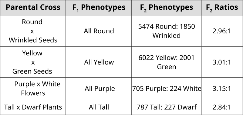
\(\newcommand{\avec}{\mathbf a}\) \(\newcommand{\bvec}{\mathbf b}\) \(\newcommand{\cvec}{\mathbf c}\) \(\newcommand{\dvec}{\mathbf d}\) \(\newcommand{\dtil}{\widetilde{\mathbf d}}\) \(\newcommand{\evec}{\mathbf e}\) \(\newcommand{\fvec}{\mathbf f}\) \(\newcommand{\nvec}{\mathbf n}\) \(\newcommand{\pvec}{\mathbf p}\) \(\newcommand{\qvec}{\mathbf q}\) \(\newcommand{\svec}{\mathbf s}\) \(\newcommand{\tvec}{\mathbf t}\) \(\newcommand{\uvec}{\mathbf u}\) \(\newcommand{\vvec}{\mathbf v}\) \(\newcommand{\wvec}{\mathbf w}\) \(\newcommand{\xvec}{\mathbf x}\) \(\newcommand{\yvec}{\mathbf y}\) \(\newcommand{\zvec}{\mathbf z}\) \(\newcommand{\rvec}{\mathbf r}\) \(\newcommand{\mvec}{\mathbf m}\) \(\newcommand{\zerovec}{\mathbf 0}\) \(\newcommand{\onevec}{\mathbf 1}\) \(\newcommand{\real}{\mathbb R}\) \(\newcommand{\twovec}[2]{\left[\begin{array}{r}#1 \\ #2 \end{array}\right]}\) \(\newcommand{\ctwovec}[2]{\left[\begin{array}{c}#1 \\ #2 \end{array}\right]}\) \(\newcommand{\threevec}[3]{\left[\begin{array}{r}#1 \\ #2 \\ #3 \end{array}\right]}\) \(\newcommand{\cthreevec}[3]{\left[\begin{array}{c}#1 \\ #2 \\ #3 \end{array}\right]}\) \(\newcommand{\fourvec}[4]{\left[\begin{array}{r}#1 \\ #2 \\ #3 \\ #4 \end{array}\right]}\) \(\newcommand{\cfourvec}[4]{\left[\begin{array}{c}#1 \\ #2 \\ #3 \\ #4 \end{array}\right]}\) \(\newcommand{\fivevec}[5]{\left[\begin{array}{r}#1 \\ #2 \\ #3 \\ #4 \\ #5 \\ \end{array}\right]}\) \(\newcommand{\cfivevec}[5]{\left[\begin{array}{c}#1 \\ #2 \\ #3 \\ #4 \\ #5 \\ \end{array}\right]}\) \(\newcommand{\mattwo}[4]{\left[\begin{array}{rr}#1 \amp #2 \\ #3 \amp #4 \\ \end{array}\right]}\) \(\newcommand{\laspan}[1]{\text{Span}\{#1\}}\) \(\newcommand{\bcal}{\cal B}\) \(\newcommand{\ccal}{\cal C}\) \(\newcommand{\scal}{\cal S}\) \(\newcommand{\wcal}{\cal W}\) \(\newcommand{\ecal}{\cal E}\) \(\newcommand{\coords}[2]{\left\{#1\right\}_{#2}}\) \(\newcommand{\gray}[1]{\color{gray}{#1}}\) \(\newcommand{\lgray}[1]{\color{lightgray}{#1}}\) \(\newcommand{\rank}{\operatorname{rank}}\) \(\newcommand{\row}{\text{Row}}\) \(\newcommand{\col}{\text{Col}}\) \(\renewcommand{\row}{\text{Row}}\) \(\newcommand{\nul}{\text{Nul}}\) \(\newcommand{\var}{\text{Var}}\) \(\newcommand{\corr}{\text{corr}}\) \(\newcommand{\len}[1]{\left|#1\right|}\) \(\newcommand{\bbar}{\overline{\bvec}}\) \(\newcommand{\bhat}{\widehat{\bvec}}\) \(\newcommand{\bperp}{\bvec^\perp}\) \(\newcommand{\xhat}{\widehat{\xvec}}\) \(\newcommand{\vhat}{\widehat{\vvec}}\) \(\newcommand{\uhat}{\widehat{\uvec}}\) \(\newcommand{\what}{\widehat{\wvec}}\) \(\newcommand{\Sighat}{\widehat{\Sigma}}\) \(\newcommand{\lt}{<}\) \(\newcommand{\gt}{>}\) \(\newcommand{\amp}{&}\) \(\definecolor{fillinmathshade}{gray}{0.9}\)Mendel’s Observations
Probability: Past Punnett Squares
Punnett Squares are convenient for predicting the outcome of monohybrid or dihybrid crosses. The expectation of two heterozygous parents is 3:1 in a single trait cross or 9:3:3:1 in a two-trait cross. Performing a three or four trait cross becomes very messy. In these instances, it is better to follow the rules of probability. Probability is the chance that an event will occur expressed as a fraction or percentage. In the case of a monohybrid cross, 3:1 ratio means that there is a \(\frac{3}{4}\) (0.75) chance of the dominant phenotype with a \(\frac{1}{4}\) (0.25) chance of a recessive phenotype.
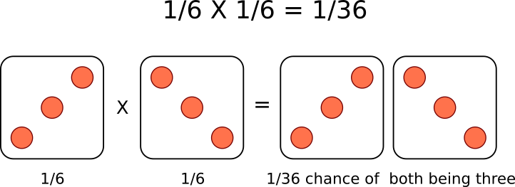
A single die has a 1 in 6 chance of being a specific value. In this case, there is a \(\frac{1}{6}\) probability of rolling a 3. It is understood that rolling a second die simultaneously is not influenced by the first and is therefore independent. This second die also has a \(\frac{1}{6}\) chance of being a 3.
We can understand these rules of probability by applying them to the dihybrid cross and realizing we come to the same outcome as the 2 monohybrid Punnett Squares as with the single dihybrid Punnett Square.
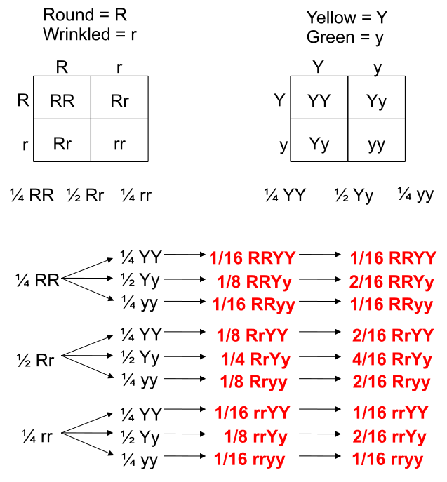
This forked line method of calculating probability of offspring with various genotypes and phenotypes can be scaled and applied to more characteristics.
The Chi-Square Test
The χ2 statistic is used in genetics to illustrate if there are deviations from the expected outcomes of the alleles in a population. The general assumption of any statistical test is that there are no significant deviations between the measured results and the predicted ones. This lack of deviation is called the null hypothesis (H0). X2 statistic uses a distribution table to compare results against at varying levels of probabilities or critical values. If the X2 value is greater than the value at a specific probability, then the null hypothesis has been rejected and a significant deviation from predicted values was observed. Using Mendel’s laws, we can count phenotypes after a cross to compare against those predicted by probabilities (or a Punnett Square).
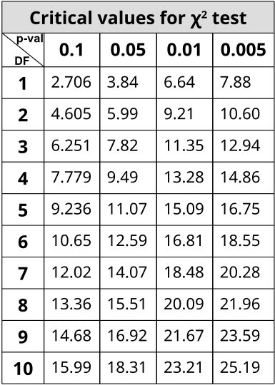
In order to use the table, one must determine the stringency of the test. The lower the p-value, the more stringent the statistics. Degrees of Freedom (DF) are also calculated to determine which value on the table to use. Degrees of Freedom is the number of classes or categories there are in the observations minus 1. DF=n-1
In the example of corn kernel color and texture, there are 4 classes: Purple & Smooth, Purple & Wrinkled, Yellow & Smooth, Yellow & Wrinkled. Therefore, DF = 4 – 1 = 3 and choosing p < 0.05 to be the threshold for significance (rejection of the null hypothesis), the X2 must be greater than 7.82 in order to be significantly deviating from what is expected. With this dihybrid cross example, we expect a ratio of 9:3:3:1 in phenotypes where 1/16th of the population are recessive for both texture and color while \(\frac{9}{16}\) of the population display both color and texture as the dominant. \(\frac{3}{16}\) will be dominant for one phenotype while recessive for the other and the remaining \(\frac{3}{16}\) will be the opposite combination.
With this in mind, we can predict or have expected outcomes using these ratios. Taking a total count of 200 events in a population, 9/16(200)=112.5 and so forth. Formally, the χ2 value is generated by summing all combinations of:
\[\frac{(Observed-Expected)^2}{Expected}\]
Chi-Square Test: Is This Coin Fair or Weighted? (Activity)
- Everyone in the class should flip a coin 2x and record the result (assumes class is 24).
- Fair coins are expected to land 50% heads and 50% tails.
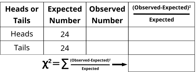
- 50% of 48 results should be 24.
- 24 heads and 24 tails are already written in the “Expected” column.
- As a class, compile the results in the “Observed” column (total of 48 coin flips).
- In the last column, subtract the expected heads from the observed heads and square it, then divide by the number of expected heads.
- In the last column, subtract the expected tails from the observed tails and square it, then divide by the number of expected tails.
- Add the values together from the last column to generate the X2 value.
- Compare the value with the value at 0.05 with DF=1.
- There are 2 classes or categories (head or tail), so DF = 2 – 1 = 1.
- Were the coin flips fair (not significantly deviating from 50:50)?
Let’s say that the coin tosses yielded 26 Heads and 22 Tails. Can we assume that the coin was unfair? If we toss a coin an odd number of times (eg. 51), then we would expect that the results would yield 25.5 (50%) Heads and 25.5 (50%) Tails. But this isn’t a possibility. This is when the X2 test is important as it delineates whether 26:25 or 30:21 etc. are within the probability for a fair coin.
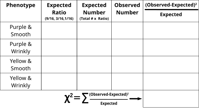
Chi-Square Test of Kernel Coloration and Texture in an F2 Population (Activity)
- From the counts, one can assume which phenotypes are dominant and recessive.
- Fill in the “Observed” category with the appropriate counts.
- Fill in the “Expected Ratio” with either 9/16, 3/16 or 1/16.
- The total number of the counted event was 200, so multiply the “Expected Ratio” x 200 to generate the “Expected Number” fields.
- Calculate the \(\frac{(Observed-Expected)^2}{Expected}\) for each phenotype combination
- Add all \(\frac{(Observed-Expected)^2}{Expected}\) values together to generate the X2 value and compare with the value on the table where DF=3.
- Do we reject the Null Hypothesis or were the observed numbers as we expected as roughly 9:3:3:1?
- What would it mean if the Null Hypothesis was rejected? Can you explain a case in which we have observed values that are significantly altered from what is expected?