5.7: Binding - Enzyme Linked Immunosorbant Assays (ELISAs)

Search Fundamentals of Biochemistry

Learning Goals (ChatGPT o1, 1/30/25)

• Fundamentals and Variants of ELISAs

  • Explain the basic principles of enzyme-linked immunosorbent assays (ELISAs) and why they are widely used in biotechnology, clinical diagnostics, and pharmaceutical research.
  • Differentiate between traditional (direct/indirect) and sandwich ELISA formats, including how each type utilizes immobilized components (antigen or antibody) and the role of secondary labeled antibodies in detection.

• Assay Design and Workflow

  • Describe the step-by-step procedure of a traditional ELISA, including antigen immobilization, blocking, addition of primary antibody, washing steps, and introduction of the secondary labeled antibody.
  • Illustrate how competition assays work (e.g., competitive ELISA) and how the presence of analyte in a test sample affects the binding dynamics and signal output.

• Detection Methods and Signal Generation

  • Identify the different labels used in ELISAs (e.g., fluorophores, enzymes) and explain how their activity (via substrate conversion) is measured using spectrophotometric or fluorometric techniques.
  • Discuss the concept of signal amplification and how it enhances assay sensitivity.

• Mathematical Modeling and Data Analysis

  • Apply the Hill equation and the logistic (4-parameter) equation to describe and analyze ELISA standard curves, including the interpretation of parameters such as the Hill coefficient, L₅₀ (or inflection point), minimum (a) and maximum (d) signal levels.
  • Evaluate how the slope of the dose–response curve (reflecting cooperativity or binding efficiency) influences data interpretation and quantitation of analyte concentration.

• Quality Control and Assay Optimization

  • Discuss key factors in ensuring ELISA reliability and validity, such as proper washing, blocking to minimize nonspecific binding, and the importance of including standard curves and appropriate controls.
  • Consider how variations in assay design (e.g., immobilization strategy, antibody pairing in sandwich ELISAs) can affect sensitivity, specificity, and dynamic range.

• Lateral Flow Immunoassays (LFAs)

  • Compare traditional ELISAs with lateral flow immunoassays, noting the differences in assay format (planar strip vs. microplate) and the role of capillary action in sample migration.
  • Explain how gold nanoparticles are used in LFAs for visual detection through surface plasmon resonance, including the underlying principles that enable observable color changes in positive tests.

By achieving these learning goals, students will be able to design, conduct, and critically evaluate immunoassays, and apply mathematical models to interpret experimental data, thereby bridging the gap between theoretical concepts and practical applications in biochemistry and related fields.

Introduction

Enzyme-linked immunosorbent assays (ELISAs) are used widely in biotechnology, pharmaceutical, and clinical medicine labs. At the same time, they appear to be underrepresented in chemistry and biochemistry curricula, even though their sensitivity, selectivity, and ease of use would argue for their widespread use.

ELISAs use primary antibodies specific to a target analyte (or antigen) as a central part of the assay. In a direct ELISA, the antigen is immobilized in wells of a multiwell plate or on a strip. An aqueous antibody solution is added, and an immobilized analyte (antigen)-antibody complex forms. After washing the bound complex on the solid phase support to remove unbound species, a second labeled antibody is added for detection. This secondary antibody binds to the bound antibody's distal end (Fc domain) and not the analyte. The label on the second antibody can either be a fluorophore or an enzyme that can interact with an added substrate that will generate a colored solution. The color development is then measured with a fluorometer or spectrophotometer.

There are several variants of ELISAs, including the traditional ELISA, in which the antigen is bound or fixed to the surface of the solid support, or a sandwich ELISA, in which the antibody is bound to the surface. In the latter case, a second labeled antibody that binds to the antigen must bind at a different site (or epitope) on the antigen. For sandwich ELISAs, the target analyte must be large enough to accommodate two antibodies binding to different sites on the same molecule.

Cartoon diagrams showing the binding interactions in traditional and sandwich ELISAs are shown in Figure \(\PageIndex{1}\).

Figure \(\PageIndex{1}\): Binding interactions in traditional and sandwich ELISAs. Abbreviations are: fixiertes (fixed or immbolized), substrat (substrate), farblos (colorless), farbig (colored), enzymegekoppelter (enyzme coupled), antikörper (antibody), zweitantikörper (second antibody), erstantikörper (primary antibody). https://commons.wikimedia.org/wiki/File:ELISA.svg. Creative Commons Attribution 4.0 International license.

Note that both types have direct and indirect versions.

Figure \(\PageIndex{2}\) shows some of the steps in a traditional ELISA.

Figure \(\PageIndex{2}\): Steps in a traditional ELISA

In (1), an analyte is added to a well (outlined in gray). The solution is removed after a predefined time, and then a specific amount of analyte (such as protein) is irreversibly adsorbed (2). A blocker, such as bovine serum albumin (BSA) or milk, is added to bind any sites on the plate that could bind protein. A primary anti-analyte protein is added. Some bind to the immobilized protein, and the rest is free in solution. After washing, only the primary antibody-immobilized analyte remains.

Now, if a test solution (for example, from a patient's blood) is added after blocking but before adding the primary antibody, it remains in the well unbound (5). If a primary antibody is added to this well, the immobilized antigen competes with the free antigen for binding, so less secondary antibody would be bound to the well (6). After washing, wells 4 and 7 remain. After additional rounds of washing and blocking, the secondary labeled antibody is added. Wells (such as 7) that contain patient analyte will bind less secondary antibody to the immobilized protein. When a substrate for the conjugated enzyme is added, the solution will be less colored after a defined incubation time.

A standard curve is made using a range of known analyte concentrations in assays. The more analytes in the standard, the greater the competition with the immobilized analyte for the solution-phase primary antibody. After washing away the solution-phase antigen:primary antibody complex, this would lead to a lower absorbance in the well with the higher solution-phase antigen in the sample.

Now, let's consider a sandwich assay. Instead of immobilizing a protein antigen, an antibody that binds the target antigen is immobilized. For example, an antibody against a surface SARS-CoV-2 protein can be immobilized. Next, a specimen (saliva, nasal swab) containing the target surface protein recognized by the immobilized antibody is added. The greater the viral load, the more SARS-CoV-2 binds to the antibody. Then, a second labeled antibody can be added that recognizes a different protein (the spike protein from SARS-CoV-2). After washing, the substrate is added, and the color development from the enzyme action on the substrate is measured. In this case, the more SARS-CoV-2 in the sample, the higher the signal (absorbance or fluorescence).

ELISAs have detection limits between 0.01 pg/mL and 100 ng/mL [1]. Although they are extensively used in health fields, they are not widely used in undergraduate biochemistry or chemistry courses, nor mentioned in the ACS’s Guidelines and Supplements for either Analytical Chemistry or Biochemistry. Given their importance, we choose to discuss them here.

ELISA Data Analysis

The most difficult parts about ELISAs are understanding the chemical and mathematical equations, choosing/using modeling and analysis software, and evaluating validity/reliability. The typical data analysis is based on the generic Hill equation instead of the classical hyperbolic binding curve analysis we derived for a single ligand to a single site on a macromolecule. The Hill equation has more empirical parameters to use when fitting bind curves.

Here is the Hill equation that we studied before.

\begin{equation}
Y=\frac{L^{n}}{K_{D}+L^{n}}
\end{equation}

For more complicated ELISA data, when a standard curve of known concentrations is used, and output signals (fluorescence, absorbance) vary from some minimum to a maximum value, a similar but more empirically useful Logistic Equation is used:

\begin{equation}
Y^{\prime}=M\left(\frac{x^{n}}{k+x^{n}}\right)
\end{equation}

where Y is the observable signal, and M is the maximal observable signal. The maximal signal might not be observed in an ELISA, as in binding a ligand to a macromolecule, when ligand concentrations >>K_D cannot be reached.

Let's use a variant of the Hill equation, using the L₅₀ value, the ligand concentration at half-maximum binding.

\begin{equation}
\begin{gathered}
0.5=\frac{L_{50}^{n}}{K_{D}+L_{50}^{n}} \\
1=\frac{2 L_{50}^{n}}{K_{D}+L_{50}{ }^{n}}
\end{gathered}
\end{equation}

hence

\begin{equation}
Y=\frac{L^{n}}{K_{D}+L^{n}}=\frac{L^{n}}{L_{50}^{n}+L^{n}}\left(\frac{\frac{1}{L^{n}}}{\frac{1}{L^{n}}}\right)=\frac{1}{\frac{L_{50}^{n}}{L^{n}}+1}=\frac{1}{\left(\frac{L_{50}}{L}\right)^{n}+1}
\end{equation}

An analogous, somewhat similar equation can be derived from the logistic equation:

\begin{equation}
Y=d+\frac{a-d}{1+\left(\frac{L}{c}\right)^{b}}
\end{equation}

where four empirical parameters define the curve:

• a is the smallest measured absorbance value (blank);
• d is the largest absorbance value when Y = 1;
• c is the inflection point in the curve, which can easily be seen to occur when [L]= L₅₀= the ligand concentration at half-maximal saturation, and
• b is the slope of the curve at L₅₀, which is the Hill coefficient n. (for many ELISA curves ≈ 1).

Figure \(\PageIndex{3}\) shows an idealized graph of ELISA data.

Figure \(\PageIndex{3}\): Idealized ELISA signal (fluorescence, absorbance) vs log [L] curve

The 4-parameter modified Logistic equation is ideal for fitting ELISA data.

An interactive active graph for the 4-parameter Logistic curve is shown in Figure \(\PageIndex{4}\). T

Figure \(\PageIndex{4}\): Interactive active graph for the four-parameter Logistic curve.

Two parameters, the minimum signal a and the maximum signal d, have been set to 0.01 and 2.0, respectively, and are not changeable in the figure. Note that the greater the value of b (slope of the curve at the inflection point), the more "sigmoidal" the semilog curve appears (similar to the Hill binding curves for hemoglobin).

Lateral flow immunoassays

During the COVID pandemic, home test kits (when they were available) were used. These tests are a modified version of the sandwich ELISA described above. They differ in two main ways. The assays were not done in wells but in a planar sheet, where the samples flowed laterally across the sheet. As it flows across a strip through capillary action, a sample containing the SARS-CoV-2 with its spike protein would first encounter a labeled antibody to the spike protein. It would then flow into a region that contained immobilized test (anti-spike protein) and control antibodies. The bound analyte would stop and build up to a sufficient concentration to see an observable colored band on the strip, but only if the sample contained the viral spike protein. These events are illustrated in Figure \(\PageIndex{5}\).

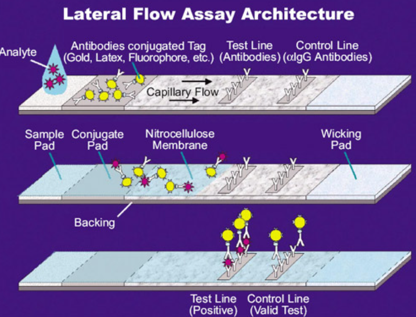
Figure \(\PageIndex{5}\): Lateral flow ELISA assay. https://en.Wikipedia.org/wiki/Latera...Flow_Assay.jpg

Figure \(\PageIndex{6}\) shows a lateral flow assay that detects the presence of serum or potentially salivary antibodies (either IgG or IgM) against the SARS-Cov2 proteins.

Figure \(\PageIndex{6}\) shows a lateral flow assay that detects the presence of serum or potentially salivary antibodies (either IgG or IgM) against the SARS-Cov2 proteins. https://commons.wikimedia.org/wiki/F...0453-g002.webp. Creative Commons Attribution 4.0 International license.

The green cube represents the virus with viral proteins. It has been labeled with a gold nanoparticle (blue sphere). Gold is widely used as a labeling reagent in lateral flow immunoassays because it is chemically inert and extremely stable. The concentrated gold particles found in positive samples at the end of the strip can be observed visually since the gold nanoparticles absorb light through surface plasmon resonance. In this process, light of specific tunable wavelengths (based on the nanoparticle size) is absorbed when it matches the oscillatory frequency of the electron clouds of the metal nanoparticle. Plasmons are the oscillations in the electrons (hence electromagnetic oscillation) that occur when the nanoparticle's surface interacts with photons, causing oscillations in the electrons at the same frequency as the light (resonance).

Gold nanoparticles (AuNPs) are used in a new (2025) assay called NasRED (Nanoparticle-Supported Rapid Electronic Detection).   The assay can detect either an antibody to a virus or bacteria, or a bacterial or viral antigen.  The assay is rapid, very sensitive, and cheap, allowing almost real-time detection (less than 15 minutes) of a sample.  The AuNPs are precoated with biotinylated antigens (to detect antibodies) or antibodies (to detect viral proteins).  A small volume sample containing the analyte is added.  The system is mixed and centrifuged so the AuNPs are sedimented.  Since the AuNPs are derivatized with multiple biotinylated sensors, the binding of antigen to the AuNPs is multivalent. Vortexing the sedimented sample resuspends the unbound AuNPs, leaving the much larger crosslinked AuNPs bound with the antigen precipitated.  The absorbance of the supernatant with unbound AnNPs is determined.  The more antigen in the sample, the fewer AuNPs in the supernatant, the lower the optical signal.

The assay requires no labeling of the sample.  It's reported to be 3000x more sensitive than an ELISA and 100Kx more sensitive than a lateral flow assay.  Imagine going to a doctor with an infection that could be viral or bacterial.  NasRED for a panel of likely infectious agents could be used, allowing almost immediate diagnosis and prescription of the appropriate antiviral or antibacterial drug.

Summary

This chapter explores the principles, methodologies, and data analysis strategies of enzyme-linked immunosorbent assays (ELISAs), a key analytical tool widely used in biotechnology, pharmaceuticals, and clinical diagnostics. Despite their widespread application in health-related fields, ELISAs have historically received less emphasis in traditional chemistry and biochemistry curricula. The chapter addresses this gap by detailing both the theoretical and practical aspects of these assays.

1. Fundamental Principles and Formats
   The chapter begins by introducing ELISAs as sensitive, selective, and user-friendly immunoassays that rely on specific antibody–antigen interactions. It reviews two primary formats:

   • Traditional ELISAs: Where the antigen is immobilized on a solid support and detected by a primary antibody followed by a secondary labeled antibody.
   • Sandwich ELISAs: Where an antibody is immobilized to capture the target antigen from a sample, and a second labeled antibody binds to a different epitope on the antigen.
     Both direct and indirect detection methods are discussed, emphasizing how enzyme or fluorophore labels generate measurable signals upon substrate conversion.

2. Assay Workflow and Mechanism
   Detailed procedural steps are outlined, including sample addition, antigen immobilization, blocking of non-specific binding sites, primary antibody incubation, and sequential washing steps that remove unbound species. The formation of an antigen–antibody complex, and subsequent binding of a labeled secondary antibody, set the stage for the detection phase. The resulting colorimetric or fluorescent signal is proportional to the amount of analyte present, enabling quantification via spectrophotometry or fluorometry.

3. Data Analysis and Mathematical Modeling
   A significant focus is placed on the analysis of ELISA data using mathematical models. The chapter contrasts classical hyperbolic binding models with the Hill equation and introduces a four-parameter logistic equation as an effective tool for fitting standard curves. Key parameters—such as the Hill coefficient (reflecting cooperativity), L₅₀ (ligand concentration at half-maximal signal), and the minimum and maximum observable signals—are defined and discussed in the context of quantifying analyte concentrations.

4. Lateral Flow Immunoassays
   Extending the discussion to point-of-care diagnostics, the chapter describes lateral flow immunoassays (LFAs), a modified version of the sandwich ELISA format adapted for use in portable, rapid test kits. The design of LFAs, which utilizes capillary action on a planar strip and gold nanoparticles for visual detection via surface plasmon resonance, is explained. This section highlights the importance of LFAs during the COVID-19 pandemic and their role in detecting viral antigens and antibodies.

5. Practical Applications and Educational Importance
   The chapter concludes by underscoring the practical significance of ELISAs and LFAs in modern laboratory settings, while also advocating for their increased incorporation into undergraduate curricula. By mastering ELISA techniques and data analysis, students gain valuable skills that bridge biochemical theory with clinical and industrial applications.

Overall, the chapter provides a comprehensive overview of ELISA technology, from its foundational concepts and assay design to advanced data modeling and real-world applications, equipping students with a thorough understanding of this essential biochemical technique.