5.7: Binding - Enzyme Linked Immunosorbant Assays (ELISAs)

Search Fundamentals of Biochemistry

Learning Goals 

(Learning goals written by Claude, Sonnet 4.6, Anthropic)

ELISA Formats and Biochemical Principles

• Compare direct, indirect, traditional, and sandwich ELISA formats in terms of which molecular species (antigen or antibody) is immobilized, how the signal is generated through enzyme-linked secondary antibody action on a chromogenic substrate, and the directional relationship between analyte concentration and signal magnitude — explaining why traditional (competitive) ELISAs give an inverse relationship while sandwich ELISAs give a direct relationship between analyte concentration and signal.
• Explain the molecular basis of blocking in ELISAs — why proteins such as BSA or milk are added after antigen or antibody immobilization — and describe how washing steps at each stage remove unbound species to reduce background while preserving the specific bound complex.
• Describe the design requirements for a sandwich ELISA — the target analyte must be large enough to present two non-overlapping epitopes simultaneously to two different antibodies — and connect this constraint to the structural features of antigens and the paratope-epitope interaction described in the antibody structure section.

Quantitative Data Analysis of ELISA and Immunoassay Signals

• Derive the four-parameter logistic equation Y = a + (d − a)/[1 + (L₅₀/L)^b] from the Hill equation framework, identify the physical meaning of each parameter (a = minimum signal, d = maximum signal, c = L₅₀ = ligand concentration at half-maximal signal, b = Hill coefficient/slope at inflection point), and explain why a semilog plot of signal vs. [analyte] produces a sigmoidal curve and why this representation is preferred over a linear concentration axis for ELISA data spanning several orders of magnitude.
• Explain how a standard curve of known analyte concentrations is used to determine the concentration of an unknown analyte in a patient sample, and identify the sources of error and limits of detection (0.01 pg/mL to 100 ng/mL) that govern the sensitivity and dynamic range of ELISA-based assays.

Lateral Flow Assays and Emerging Immunoassay Technologies

• Describe the architecture and flow sequence of a lateral flow immunoassay — sample pad, labeled antibody conjugate pad, nitrocellulose membrane with test and control lines — explaining how capillary action drives the sample across the strip, how a positive result produces a visible test band through accumulation of gold nanoparticle-labeled analyte:antibody complexes, and why a control line is essential for assay validation.
• Explain the physical basis of gold nanoparticle detection by surface plasmon resonance — collective oscillations of the conduction electron cloud at the nanoparticle surface driven to resonance by photons of matching frequency — and describe why gold nanoparticles are preferred as lateral flow labels (chemical inertness, stability, tunable absorption wavelength based on particle size, and visual detectability at concentrations achievable in positive samples).
• Describe the NasRED (Nanoparticle-Supported Rapid Electronic Detection) assay principle — multivalent binding of analyte to biotinylated AuNPs causes crosslinking and precipitation of large AuNP aggregates, reducing supernatant absorbance in proportion to analyte concentration — and compare its sensitivity (~3000× more sensitive than ELISA, ~100,000× more sensitive than lateral flow assays), speed (<15 minutes), and cost relative to conventional immunoassays, explaining the clinical significance for rapid differential diagnosis of viral vs. bacterial infection

Introduction

Enzyme-linked immunosorbent assays (ELISAs) are used widely in biotechnology, pharmaceutical, and clinical medicine labs. At the same time, they appear underrepresented in chemistry and biochemistry curricula, even though their sensitivity, selectivity, and ease of use would argue for their widespread adoption.

ELISAs use primary antibodies specific to a target analyte (or antigen) as a central part of the assay. In a direct ELISA, the antigen is immobilized in wells of a multiwell plate or on a strip. An aqueous antibody solution is added, and an immobilized analyte (antigen)-antibody complex forms. After washing the complex bound to the solid-phase support to remove unbound species, a second labeled antibody is added for detection. This secondary antibody binds to the distal end of the bound antibody (the Fc domain), not the analyte. The label on the second antibody can be a fluorophore or an enzyme that interacts with an added substrate to generate a colored solution. The color development is then measured with a fluorometer or spectrophotometer.

There are several variants of ELISAs, including the traditional ELISA, in which the antigen is bound to or immobilized on the solid support, and the sandwich ELISA, in which the antibody is bound to the solid support. In the latter case, a second labeled antibody that binds to the antigen must bind at a different site (or epitope) on the antigen. For sandwich ELISAs, the target analyte must be large enough to accommodate two antibodies binding to different sites on the same molecule.

Cartoon diagrams showing the binding interactions in traditional and sandwich ELISAs are shown in Figure \(\PageIndex{1}\).

Figure \(\PageIndex{1}\): Binding interactions in traditional and sandwich ELISAs. Abbreviations are: fixiertes (fixed or immbolized), substrat (substrate), farblos (colorless), farbig (colored), enzymegekoppelter (enyzme coupled), antikörper (antibody), zweitantikörper (second antibody), erstantikörper (primary antibody). https://commons.wikimedia.org/wiki/File:ELISA.svg. Creative Commons Attribution 4.0 International license.

Note that both types have direct and indirect versions.

Figure \(\PageIndex{2}\) shows some of the steps in a traditional ELISA.

Figure \(\PageIndex{2}\): Steps in a traditional ELISA

In (1), an analyte is added to a well (outlined in gray). The solution is removed after a predefined time, and then a specific amount of analyte (such as protein) is irreversibly adsorbed (2). A blocker, such as bovine serum albumin (BSA) or milk, is added to bind any sites on the plate that could bind protein. A primary anti-analyte protein is added. Some bind to the immobilized protein, and the rest is free in solution. After washing, only the analyte immobilized with the primary antibody remains.

Now, if a test solution (for example, from a patient's blood) is added after blocking but before adding the primary antibody, it remains in the well unbound (5). If a primary antibody is added to this well, the immobilized antigen competes with free antigen for binding, so less secondary antibody would bind to the well (6). After washing, wells 4 and 7 remain. After additional rounds of washing and blocking, the secondary antibody labeled with a fluorophore is added. Wells (such as 7) that contain patient analyte will bind less secondary antibody to the immobilized protein. When a substrate for the conjugated enzyme is added, the solution will be less colored after a defined incubation time.

A standard curve is made using a range of known analyte concentrations in assays. The more analytes in the standard, the greater the competition for the solution-phase primary antibody between the immobilized analyte and the analytes in the standard. After washing away the solution-phase antigen:primary antibody complex, this would lead to a lower absorbance in the well with the higher solution-phase antigen in the sample.

Now, let's consider a sandwich assay. Instead of immobilizing a protein antigen, an antibody that binds the target antigen is immobilized. For example, an antibody against a surface SARS-CoV-2 protein can be immobilized. Next, a specimen (saliva, nasal swab) containing the target surface protein recognized by the immobilized antibody is added. The greater the viral load, the more SARS-CoV-2 binds to the antibody. Then, a second labeled antibody can be added that recognizes a different protein (the spike protein from SARS-CoV-2). After washing, the substrate is added, and the color development from the enzyme action on the substrate is measured. In this case, the more SARS-CoV-2 in the sample, the higher the signal (absorbance or fluorescence).

ELISAs have detection limits ranging from 0.01 pg/mL to 100 ng/mL [1]. Although they are extensively used in health fields, they are not widely used in undergraduate biochemistry or chemistry courses, nor are they mentioned in the ACS’s Guidelines and Supplements for either Analytical Chemistry or Biochemistry. Given their importance, we choose to discuss them here.

ELISA Data Analysis

The most difficult parts about ELISAs are understanding the chemical and mathematical equations, choosing/using modeling and analysis software, and evaluating validity/reliability. Typical data analysis is based on the generic Hill equation rather than the classical hyperbolic binding curve analysis we derived for a single ligand binding to a single site on a macromolecule. The Hill equation has more empirical parameters for fitting binding curves.

Here is the Hill equation that we studied before.

\begin{equation}
Y=\frac{L^{n}}{K_{D}+L^{n}}
\end{equation}

For more complicated ELISA data, when a standard curve of known concentrations is used and output signals (fluorescence, absorbance) vary from some minimum to a maximum value, a similar but more empirically useful Logistic Equation is used:

\begin{equation}
Y^{\prime}=M\left(\frac{x^{n}}{k+x^{n}}\right)
\end{equation}

where Y is the observable signal, and M is the maximal observable signal. The maximal signal might not be observed in an ELISA, as in binding a ligand to a macromolecule, when ligand concentrations >>K_D cannot be reached.

Let's use a variant of the Hill equation based on the L₅₀ value, the ligand concentration at half-maximum binding.

\begin{equation}
\begin{gathered}
0.5=\frac{L_{50}^{n}}{K_{D}+L_{50}^{n}} \\
1=\frac{2 L_{50}^{n}}{K_{D}+L_{50}{ }^{n}}
\end{gathered}
\end{equation}

hence

\begin{equation}
Y=\frac{L^{n}}{K_{D}+L^{n}}=\frac{L^{n}}{L_{50}^{n}+L^{n}}\left(\frac{\frac{1}{L^{n}}}{\frac{1}{L^{n}}}\right)=\frac{1}{\frac{L_{50}^{n}}{L^{n}}+1}=\frac{1}{\left(\frac{L_{50}}{L}\right)^{n}+1}
\end{equation}

An analogous, somewhat similar equation can be derived from the logistic equation:

\begin{equation}
Y=d+\frac{a-d}{1+\left(\frac{L}{c}\right)^{b}}
\end{equation}

where four empirical parameters define the curve:

• a is the smallest measured absorbance value (blank);
• d is the largest absorbance value when Y = 1;
• c is the inflection point in the curve, which can easily be seen to occur when [L]= L₅₀= the ligand concentration at half-maximal saturation, and
• b is the slope of the curve at L₅₀, which is the Hill coefficient n. (for many ELISA curves ≈ 1).

Figure \(\PageIndex{3}\) shows an idealized graph of ELISA data.

Figure \(\PageIndex{3}\): Idealized ELISA signal (fluorescence, absorbance) vs log [L] curve

The 4-parameter modified Logistic equation is ideal for fitting ELISA data.

An interactive active graph for the 4-parameter Logistic curve is shown in Figure \(\PageIndex{4}\). T

Figure \(\PageIndex{4}\): Interactive active graph for the four-parameter Logistic curve.

Two parameters, the minimum signal a and the maximum signal d, have been set to 0.01 and 2.0, respectively, and are not changeable in the figure. Note that the greater the value of b (slope of the curve at the inflection point), the more "sigmoidal" the semilog curve appears (similar to the Hill binding curves for hemoglobin).

Lateral flow immunoassays

During the COVID pandemic, home test kits (when they were available) were used. These tests are a modified version of the sandwich ELISA described above. They differ in two main ways. The assays were not performed in wells but on a planar sheet, where the samples flowed laterally across it. As it flows across a strip through capillary action, a sample containing SARS-CoV-2 with its spike protein would first encounter a labeled antibody to the spike protein. It would then flow into a region that contained immobilized test (anti-spike protein) and control antibodies. The bound analyte would stop and build up to a sufficient concentration to see an observable colored band on the strip, but only if the sample contained the viral spike protein. These events are illustrated in Figure \(\PageIndex{5}\).

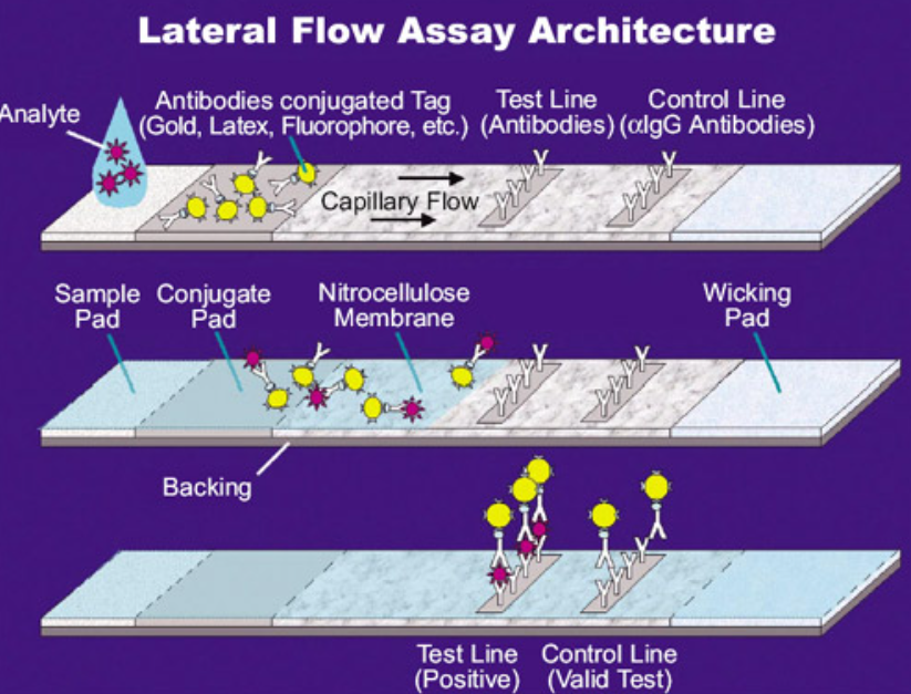
Figure \(\PageIndex{5}\): Lateral flow ELISA assay. https://en.Wikipedia.org/wiki/Latera...Flow_Assay.jpg

Figure \(\PageIndex{6}\) shows a lateral flow assay that detects the presence of serum or potentially salivary antibodies (either IgG or IgM) against the SARS-CoV-2 proteins.

Figure \(\PageIndex{6}\) shows a lateral flow assay that detects the presence of serum or potentially salivary antibodies (either IgG or IgM) against the SARS-Cov2 proteins. https://commons.wikimedia.org/wiki/F...0453-g002.webp. Creative Commons Attribution 4.0 International license.

The green cube represents the virus, including its viral proteins. It has been labeled with a gold nanoparticle (blue sphere). Gold is widely used as a labeling reagent in lateral flow immunoassays because it is chemically inert and extremely stable. The concentrated gold particles found in positive samples can be observed visually since the gold nanoparticles absorb light through surface plasmon resonance. In this process, light at specific tunable wavelengths (depending on nanoparticle size) is absorbed when it matches the oscillatory frequency of the metal nanoparticle's electron clouds. Plasmons are the oscillations in the electrons (hence electromagnetic oscillation) that occur when the nanoparticle's surface interacts with photons, causing oscillations in the electrons at the same frequency as the light (resonance).

Gold nanoparticles (AuNPs) are used in a new (2025) assay called NasRED (Nanoparticle-Supported Rapid Electronic Detection).   The assay can detect either an antibody to a virus or bacteria, or a bacterial or viral antigen.  The assay is rapid, highly sensitive, and inexpensive, allowing almost real-time detection of a sample (less than 15 minutes).  The AuNPs are precoated with biotinylated antigens (to detect antibodies) or antibodies (to detect viral proteins).  A small volume sample containing the analyte is added.  The system is mixed and centrifuged to sediment the AuNPs.  Since the AuNPs are derivatized with multiple biotinylated sensors, the binding of antigen to the AuNPs is multivalent. Vortexing the sedimented sample resuspends the unbound AuNPs, leaving the much larger crosslinked AuNPs bound with the antigen precipitated.  The absorbance of the supernatant with unbound AuNPs is determined.  The more antigen in the sample, the fewer AuNPs in the supernatant, the lower the optical signal.

The assay requires no sample labeling.  It's reported to be 3000x more sensitive than an ELISA and 100Kx more sensitive than a lateral flow assay.  Imagine going to a doctor with an infection that could be viral or bacterial.  NasRED, designed for a panel of likely infectious agents, could enable almost immediate diagnosis and prescription of the appropriate antiviral or antibacterial drug.

Summary

(Summary written by Claude, Sonnet 4.6, Anthropic)

This chapter applies the principles of antibody-antigen binding established in earlier sections to the practical context of immunoassay technology — describing how the specificity and affinity of antibody:antigen interactions are harnessed for the quantitative detection of analytes in complex biological samples, how ELISA data are analyzed mathematically, and how lateral flow and emerging nanoparticle-based platforms extend these capabilities toward rapid, sensitive, point-of-care diagnostics.

ELISA principles and formats rest on three key features shared by all variants: the immobilization of one binding partner (antigen or antibody) on a solid phase to enable washing away of unbound species; the use of a secondary antibody conjugated to an enzyme (such as horseradish peroxidase or alkaline phosphatase) whose action on a chromogenic substrate converts a binding event into a quantifiable optical signal; and blocking of non-specific protein-binding sites on the solid support with inert proteins (BSA, milk) to minimize background. In a traditional (competitive) ELISA, antigen is immobilized, and the unknown sample competes with the immobilized antigen for binding to the primary antibody — the more antigen in the sample, the less primary antibody binds to the plate, the less secondary antibody is subsequently bound, and the lower the final signal. In a sandwich ELISA, a capture antibody is immobilized, and the analyte is "sandwiched" between two antibodies binding at distinct, non-overlapping epitopes; the signal is directly proportional to analyte concentration, making this format more sensitive and suitable for large antigens. Both formats have direct (primary antibody is labeled) and indirect (secondary antibody is labeled) variants. The indirect format amplifies the signal because multiple secondary antibodies can bind to each primary antibody.

ELISA data analysis uses the four-parameter logistic (4PL) equation rather than a simple hyperbolic binding function, because ELISA signals span a sigmoidal range in semi-logarithmic space. The equation Y = a + (d − a)/[1 + (L50/[L])^b] contains four empirically determined parameters: a (minimum background signal when no analyte is present), d (maximum signal at saturating analyte concentration), c = L₅₀ (the analyte concentration at the inflection point, equivalent to the EC₅₀ or half-maximal signal concentration), and b (the slope at the inflection point, analogous to the Hill coefficient n, often ≈ 1 for typical ELISAs but greater than 1 for more cooperative systems). A standard curve — signal plotted against log[analyte] for a series of known concentrations — produces a characteristic sigmoidal curve whose inflection point and slope are determined by nonlinear regression fitting. Unknown concentrations are interpolated from the standard curve. Detection limits range from ~0.01 pg/mL to ~100 ng/mL depending on antibody affinity and assay format, making ELISAs far more sensitive than many conventional analytical methods.

Lateral flow immunoassays (familiar from COVID-19 home test kits) apply the sandwich ELISA principle to a planar format where capillary action drives the sample across a nitrocellulose membrane. The sample first encounters labeled antibody conjugated to gold nanoparticles (AuNPs) in the conjugate pad; if the target analyte (e.g., the SARS-CoV-2 spike protein) is present, it forms a complex with the labeled antibody. This complex then flows into the test zone, where an immobilized capture antibody recognizes a distinct epitope on the analyte, concentrating the AuNP-labeled complexes into a visible band. A separate control line captures excess labeled antibody to confirm adequate sample flow regardless of analyte presence. The visual detection is enabled by surface plasmon resonance of the AuNPs: incident photons whose frequency matches the collective oscillatory resonance of the gold conduction electrons at the nanoparticle surface are absorbed, producing the characteristic red color visible at the test and control lines. Gold is preferred because it is chemically inert, extremely stable, and has an absorption wavelength that can be tuned by particle size.

A major emerging innovation is NasRED (Nanoparticle-Supported Rapid Electronic Detection), a 2025-developed assay in which AuNPs precoated with biotinylated antigens (or antibodies) bind analyte through multivalent interactions. Analyte binding crosslinks multiple AuNPs into large aggregates that are sedimented by centrifugation, while unbound single AuNPs remain in suspension. Measuring the absorbance of the supernatant quantifies the unbound AuNP fraction — the more analyte present, the more AuNPs aggregate and sediment, and the lower the supernatant absorbance. This approach requires no sample labeling, is completed in under 15 minutes, and achieves a sensitivity approximately 3,000-fold greater than conventional ELISA and 100,000-fold greater than lateral flow assays. For clinical practice, a NasRED panel targeting common viral and bacterial pathogens could enable near-real-time differential diagnosis at the point of care, allowing immediate selection of appropriate antiviral or antibacterial therapy rather than empirical treatment — a significant advance in personalized infectious disease management.