4.12: Laboratory Determination of the Thermodynamic Parameters for Protein Denaturation

Search Fundamentals of Biochemistry

Learning Goals (ChatGPT o1, 1/27/25)

1. Comprehend Experimental Methods:

   • Explain how various techniques (UV absorbance, fluorescence, circular dichroism, and viscosity measurements) are used to monitor protein denaturation as a function of temperature or denaturant concentration.
   • Describe what each observable (e.g., A₂₈₀, fluorescence intensity) indicates about the protein’s conformational state.

2. Quantitative Analysis of Denaturation Curves:

   • Derive and interpret the equation y=f_Ny_N+f_Dy_D and show how to calculate the fraction denatured (f_D) using the equation f_D=y−y_Ny_D−y_N.
   • Relate the fractional denaturation to the equilibrium constant for the unfolding reaction: K_eq=f_D/(1−f_D)

3. Thermodynamic Calculations of Protein Stability:

   • Use the relationship ΔG⁰=−RTln⁡K_eq = -RTlnK[f_D/(1-f_D] to calculate the standard free energy of unfolding from experimental data.
   • Explain how ΔG⁰ changes with temperature and denaturant concentration, and describe what conditions yield ΔG⁰ = 0 (the melting temperature, Tₘ).

4. Understanding Denaturant Effects:

   • Interpret the linear relationship ΔG⁰=ΔG_w⁰−m[urea] and explain how the extrapolation to [urea] = 0 gives the free energy of unfolding in water (ΔG_w⁰).

5. Thermal Denaturation and van ’t Hoff Analysis:

   • Analyze thermal denaturation data to construct a van ’t Hoff plot (ln⁡K_eq versus 1/T) and extract ΔH⁰ and ΔS⁰ from the slope and intercept, respectively.
   • Compare van ’t Hoff enthalpy (ΔH_vHoff) with calorimetric enthalpy (ΔH_cal) obtained from differential scanning calorimetry.

6. Critical Evaluation of Data and Models:

   • Evaluate the assumptions behind a two-state model for protein unfolding and discuss the potential presence of intermediates.
   • Understand the limitations of extrapolating data (e.g., long extrapolation of ΔG⁰ to zero denaturant and infinite temperature considerations in van ’t Hoff analysis).

7. Application to Protein Mutagenesis:

   • Explain how changes in the calculated ΔG⁰ (or ΔΔG) for protein mutants can be used to assess alterations in protein stability under physiological conditions.

These learning goals aim to equip you with the conceptual and quantitative tools needed to analyze protein stability through experimental denaturation data and thermodynamic principles.

Introduction

Multiple methods can be used to investigate the denaturation of a protein. These include UV, fluorescence, CD, and viscosity measurements. In all these methods, the dependent variable (y) is measured as a function of the independent variable, which is often temperature (for thermal denaturation curves) or denaturant (such as urea, guanidine hydrochloride) concentration. From these curves, we want to calculate the standard free energy of unfolding (ΔG^O) for the protein (for the reaction N ↔ D). It is relatively easy to calculate if the denaturation curves show a sigmoidal, cooperative transition from the native to the denatured state, indicating a two-state transition. The dependent variable can also be normalized to show fractional denaturation (fD). An idealized denaturation curve is shown below in Figure \(\PageIndex{1}\).

Figure \(\PageIndex{1}\): Graphical analysis of protein denaturation

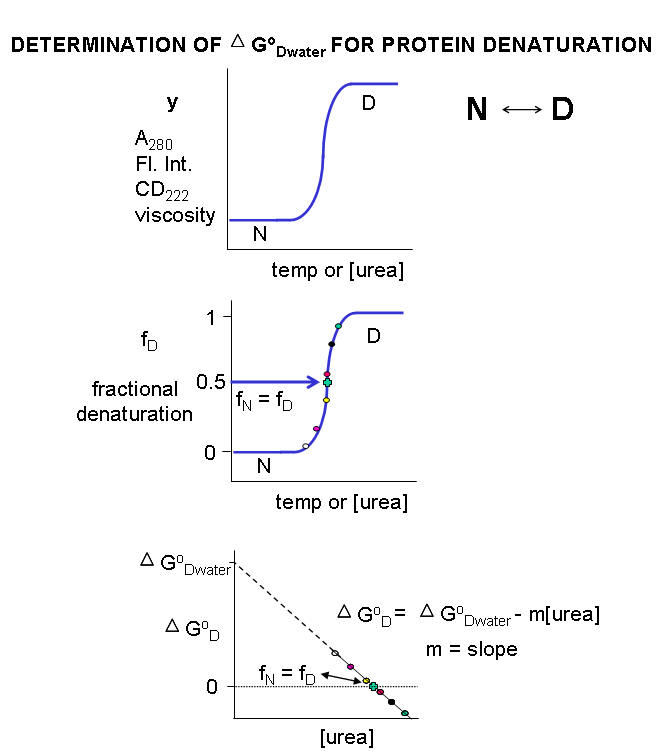
A more realistic denaturation curve might show a small linear change in the dependent variable (fluorescence intensity, for example) for temperature or denaturant concentrations well before the major unfolding transition and above those at which it is unfolded. In these cases, the mathematical analyses presented at the end are required.

Denaturation with urea or guanidine hydrochloride

For each curve, the value of y (either A₂₈₀, fluorescence intensity, viscosity, etc.) can be considered the sum contributed by the native state and the denatured states, which are both present in different fractional concentrations from 0 - 1. Hence, the following equation should be reasonably intuitive.

\begin{equation}
y=\left(f_N y_N\right)+\left(f_D y_D\right)
\end{equation}

where f_N is the fraction native and y_N is the contribution to the dependent variable y from the native state, and f_D is the fraction denatured and y_D is the contribution to the dependent variable y from the denatured state. Conservation gives the following equation.

\begin{equation}
1=f_N+f_D \text { or } f_N=1-f_D
\end{equation}

Substituting (2) into (1) gives

\begin{equation}
y=\left(1-f_D\right) y_N+\left(f_D y_D\right)=y_N-f_D y_N+\left(f_D y_D\right)
\end{equation}

Rearranging this equation gives

\begin{equation}
\mathrm{f}_{\mathrm{D}}=\frac{\mathrm{y}-\mathrm{y}_{\mathrm{N}}}{\mathrm{y}_{\mathrm{D}}-\mathrm{y}_{\mathrm{N}}}
\end{equation}

Notice the right-hand side of the equations contains variables that are easily measured.

By substituting (2) and (3) into the expression for the equilibrium constant for the reaction N <=> D we get:

\begin{equation}
K_{e q}=\frac{[D]_{e q}}{[N]_{e q}}=\frac{f_D}{f_N}=\frac{f_D}{1-f_D}
\end{equation}

From this, we can calculate ΔG⁰.

\begin{equation}
\Delta \mathrm{G}^0=-\mathrm{R} \operatorname{Tln} \mathrm{~K}_{\mathrm{eq}}=-\mathrm{R} \operatorname{Tln}\left[\frac{\mathrm{f}_{\mathrm{D}}}{1-\mathrm{f}_{\mathrm{D}}}\right]
\end{equation}

Remember that ΔG^O (and hence K_eq) depends only on the intrinsic stability of the native vs denatured state for a given set of conditions. They vary as a function of temperature and solvent conditions. At low temperatures and low urea/guanidine HCl concentration, the native state is favored, and for the N ↔ D transition, ΔG^O > 0 (i.e., denaturation is NOT favored). The denatured state is favored at high temperatures and urea/guanidine-HCl concentrations and ΔG^O < 0.

At some temperature or urea/guanidine concentration value, both the native and denatured states would be equally favored. At this value, K_eq = 1 and ΔG^O = 0.

The temperature at the maximal C_p value is called the protein's melting temperature (Tm). It is analogous to the T_m in the heat capacity vs temperature graphs for protein denaturation, as we saw in Chapter 4.9. This is Illustrated in Figure \(\PageIndex{2}\).

Figure \(\PageIndex{2}\): T_m for thermal denaturation of a protein

Ordinarily, at a temperature much below the T_m for the protein or at a low urea concentration, so little of the protein would be in the D state that it would be extremely difficult to determine the protein concentration in the D state. Hence, it would be difficult to determine the K_eq or ΔG^o for the reaction N ↔ D. However, in the range where the protein denatures (either with urea or increasing temperature), it is possible to measure f_D/f_N.and hence ΔG^o at each urea or temperature.

Now, we can calculate the ΔG^o_w for N ↔ D in water without urea. For a simple two-state N ↔ D, a plot of ΔG^o vs [urea] is linear and given by the following equation, which should be evident from (\PageIndex{1}\).

\begin{equation}
\Delta \mathrm{G}^0=\Delta \mathrm{G}_{\mathrm{w}}^0-\mathrm{m}[\text { urea }]
\end{equation}

It is important to know the K_eq and ΔG⁰ for the N ↔ D transition without urea and under "physiological conditions." A comparison of the calculated values of ΔG⁰_w in the absence of urea for a series of similar proteins (such as those varying by a single amino acid prepared by site-specific mutagenesis of the normal or wild-type gene, would indicate to what extent the mutants were stabilized or destabilized compared to the wild-type protein. ΔG⁰_w for the N ↔ D transition of the protein in the absence of denaturant (i.e., in water) can be determined by extrapolating the straight line to [urea] = 0. Admittedly, this is a long extrapolation, but reasonable values can be obtained with high-quality data and a high correlation coefficient for the linear regression analysis of the best-fit line.

Denaturation with heat

Calculation of ΔH^o and ΔS^o for N <=>D at room temperature

K_eq values can be calculated from thermal denaturation curves as described above using urea as a denaturant by monitoring change in an observable (spectra signal, for example) vs. temperature. Knowing K_eq and ΔH⁰, DS⁰ can be calculated from the equation below since a semi-log plot of lnK_eq vs 1/T is a straight line with a slope of - ΔH⁰R and a y-intercept of + ΔS⁰/R, where R is the ideal gas constant.

\begin{equation}
\begin{gathered}
\Delta \mathrm{G}^{0}=\Delta \mathrm{H}^{0}-\mathrm{T} \Delta \mathrm{S}^{0}=-\mathrm{RTln} \mathrm{K}_{\mathrm{eq}} \\
\ln \mathrm{K}_{\mathrm{eq}}=-\frac{\Delta \mathrm{H}^{0}-\mathrm{T} \Delta \mathrm{S}^{0}}{\mathrm{RT}} \\
\ln \mathrm{K}_{\mathrm{eq}}=-\frac{\Delta \mathrm{H}^{0}}{\mathrm{RT}}+\frac{\Delta \mathrm{S}^{0}}{\mathrm{R}}
\end{gathered}
\end{equation}

From these equations, it should be evident that all the major thermodynamics constants (ΔG⁰, ΔH⁰ and ΔS⁰ ) for the N ↔ D transition can be calculated from thermal denaturation curves.

Equation (8) below shows that the derivative of equation (7) with respect to 1/T (i.e. the slope of equation 7 plotted as lnK_eq vs 1/T) is indeed -ΔH⁰/R. Equation (8) is the van 't Hoff equation, and the calculated value of the enthalpy change is termed the van 't Hoff enthalpy, ΔH⁰v_Hoff.

\begin{equation}
\frac{d \ln \mathrm{K}_{\mathrm{eq}}}{d(1 / \mathrm{T})}=-\frac{\Delta \mathrm{H}^{0}}{\mathrm{R}}=-\frac{\Delta \mathrm{H}_{\mathrm{vHoff}}^{0}}{\mathrm{R}}
\end{equation}

It is helpful to compare the van 't Hoff enthalpy, ΔH⁰v_Hoff, with the enthalpy change determined directly using differential scanning calorimetry by analyzing a plot of Cp vs T. (Note that the area under the Cp vs T curve, as the protein transitions to the unfolded state, has units of kcal or kJ. The ΔH⁰ for the unfolding is inversely proportional to the width of the curve.)

In contrast to the long extrapolation of the ΔG⁰ vs [urea] to [urea] = 0 to get ΔG⁰ (the y-intercept) in the absence of urea, which has some physical meaning, extrapolation of the straight line from the van 't Hoff plot from equation 8 to get ΔS⁰/R, the y-intercept, has little meaning since the 1/T value at the y-intercept is 0, which occurs when T approaches infinity. ΔS⁰ can be calculated at any reasonable temperature from the calculated value of ΔG⁰ at that temperature and the calculated ΔH⁰_vHoff.

Summary

This chapter delves into how we quantify and understand protein stability through thermodynamic principles and experimental measurements. We begin by recognizing that protein stability is a delicate balance between favorable interactions (such as hydrophobic effects, hydrogen bonds, and van der Waals forces) that stabilize the native state and the inherent conformational entropy of the polypeptide chain that favors the denatured state.

To investigate these factors, various experimental methods—including UV absorbance, fluorescence, circular dichroism (CD), and viscosity measurements—are used to monitor the unfolding transition of proteins. By analyzing denaturation curves (plotted as a function of temperature or denaturant concentration), we can determine the fraction of protein in the native versus the denatured state. The relationship

y=f_Ny_N+f_Dy_D and f_D=y−y_Ny_D−y_N

allows us to quantify the fraction denatured (fDf_D) based on an observable yy (e.g., absorbance or fluorescence intensity). From there, the equilibrium constant for unfolding, K_eq=f_D/(1−f_D), leads directly to calculating the standard free energy change for unfolding (ΔG⁰=−RTln⁡K_eq.

For thermal denaturation, the melting temperature (Tm) is defined as the point where half of the protein population is unfolded (i.e., K_eq=1 and ΔG⁰=0). By constructing van ’t Hoff plots (lnK_eq vs. 1/T₁), we can extract the enthalpy (ΔH⁰) and entropy (ΔS⁰) changes associated with protein unfolding. These thermodynamic parameters are crucial for understanding how proteins respond to environmental changes and how mutations might alter protein stability.

Finally, the chapter emphasizes the importance of rigorous data analysis and careful extrapolation of denaturation curves to obtain accurate estimates of protein stability under physiological conditions. Such quantitative assessments provide a foundation for comparing the stability of wild-type proteins with mutant forms and for understanding the molecular forces that drive protein folding and function.

This integrated thermodynamic framework equips you with the conceptual and analytical tools necessary to interpret experimental data and to appreciate the fine balance that maintains protein structure and function.