22.5: Measuring Biodiveristy

Diversity Indices

A diversity index is a quantitative measure that reflects how many different types (such as species) there are in a dataset (a community). These indices are statistical representations of biodiversity in different aspects (richness, evenness, and dominance). When diversity indices are used in ecology, the types of interest are usually species, but they can also be other categories, such as genera, families, functional types, or haplotypes. The entities of interest are usually individual plants or animals, and the measure of abundance can be, for example, number of individuals, biomass or coverage.

Richness simply quantifies how many different types the dataset of interest contains. For example, species richness (usually noted S) of a dataset is the number of species in the corresponding species list. Richness is a simple measure, so it has been a popular diversity index in ecology, where abundance data are often not available for the datasets of interest. 

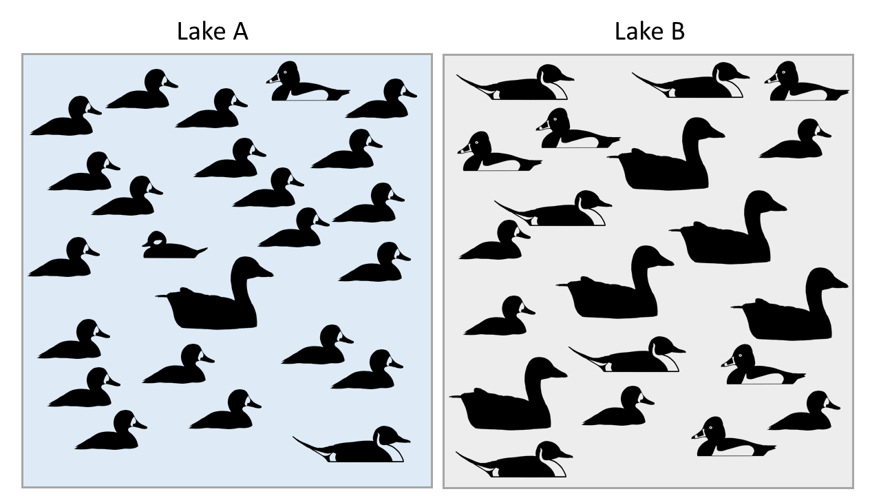
Although species richness (denoted S) is often used as a measure of biodiversity, of more interest to ecologists and conservation biologists are diversity indices that include both species richness and measures of abundance. This is because richness alone does not account for evenness across species. In example 22.2.1 below, both lakes have the same richness, but Lake B is more diverse because abundance is spread more evenly across the species present. 

Many different indices of diversity are used by scientists, but below we cover the most widely used.

Simpson’s Index

Simpson (1949) developed an index of diversity which is a measure of probability--the less diversity, the greater the probability that two randomly selected individuals will be the same species. In the absence of diversity (1 species), the probability that two individuals randomly selected will be the same is 1. Simpson's Index is calculated as follows:

\[D=\sum_{i=1}^{S}\left(\frac{n_{i}}{N}\right)^{2}\]

where n_i is the number of individuals in species i, N = total number of individuals of all species, and n_i/N = p_i (proportion of individuals of species i), and S = species richness.

The value of Simpson’s D ranges from 0 to 1, with 0 representing infinite diversity and 1 representing no diversity, so the larger the value of D, the lower the diversity. For this reason, Simpson’s index is often as its complement (1-D). Simpson's Dominance Index is the inverse of the Simpson's Index (1/D). 

Shannon-Weiner Index

Another widely used index of diversity that also considers both species richness and evenness is the Shannon-Weiner Diversity Index, originally proposed by Claude Shannon in 1948. It is also known as Shannon's diversity index. The index is related to the concept of uncertainty. If for example, a community has very low diversity, we can be fairly certain of the identity of an organism we might choose by random (high certainty or low uncertainty). If a community is highly diverse and we choose an organism by random, we have a greater uncertainty of which species we will choose (low certainty or high uncertainty).

\[H=-\sum_{i=1}^{S} p_{i} * \ln p_{i}\]

where p_i = proportion of individuals of species i, and ln is the natural logarithm, and  S = species richness.

The value of H ranges from 0 to H_max. H_max is different for each community and depends on species richness. (Note: Shannon-Weiner is often denoted H' ).

Evenness Index

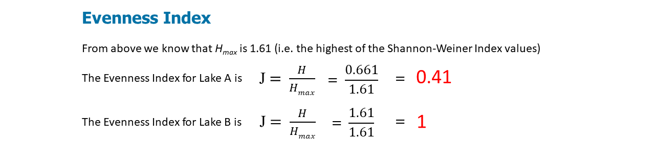
Species evenness refers to how close in numbers each species in an environment is. So if there are 40 foxes and 1000 dogs, the community is not very even. But if there are 40 foxes and 42 dogs, the community is quite even. The evenness of a community can be represented by Pielou's evenness index (Pielou 1966):

\[J=\frac{H}{H_{\max }}\]

The value of J ranges from 0 to 1. Higher values indicate higher levels of evenness. At maximum evenness, J = 1.

J and D can be used as measures of species dominance (the opposite of diversity) in a community. Low J indicates that 1 or few species dominate the community.

Example \(\PageIndex{1}\)

Calculate Simpson's Index, Shannon-Weiner Index, and the Evenness Index for waterbirds on two lakes: Lake A, and Lake B. There are 5 species and 25 individuals on both lakes, but are they equally diverse?

Here are the solutions:

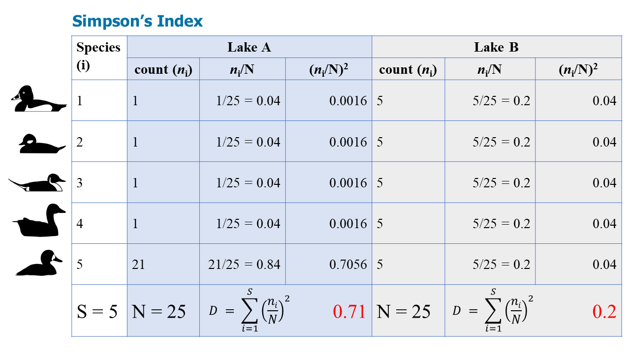
Note that Simpson's Index is often expressed (1-D), so the final answers are 0.29 and 0.8. This makes more intuitive sense: a higher D is more diverse--which is Lake B because it is less dominated by one species.

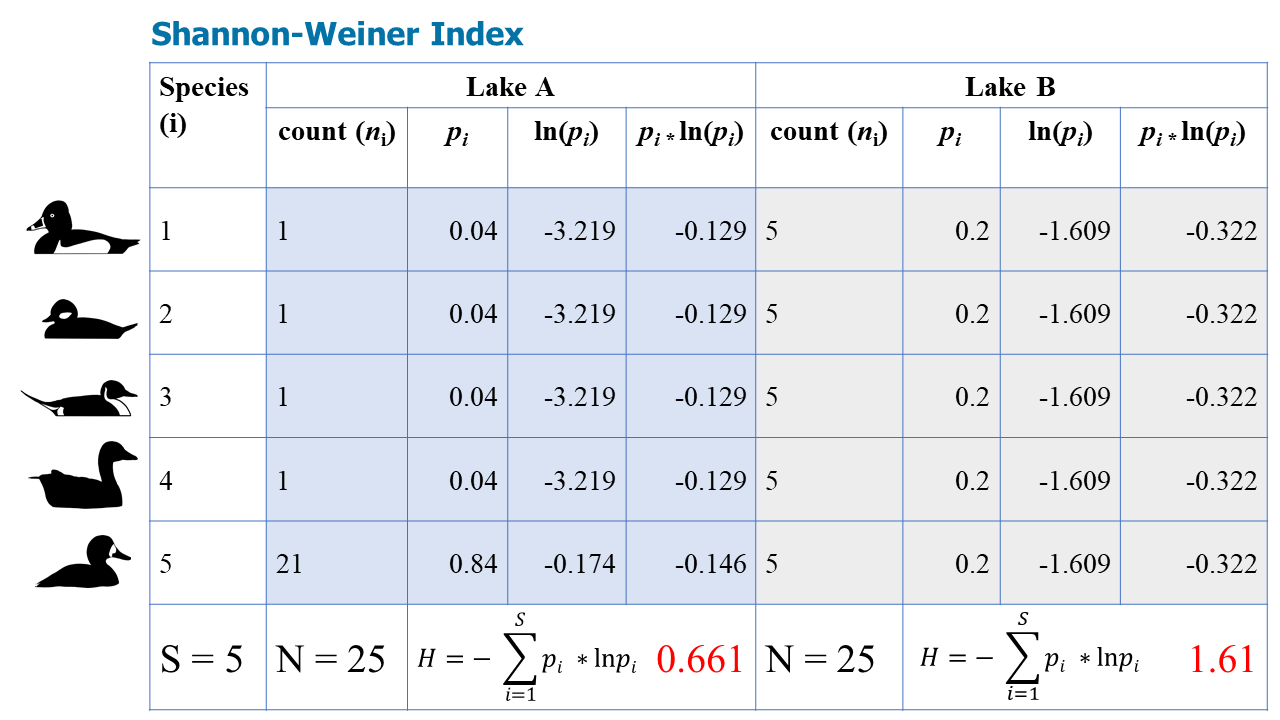
Again, according to the Shannon-Weiner Index, Lake B is more diverse.

Conclusion

By all three measures, Lake B is more diverse, despite the fact that the two lakes have identical species richness.

Rarefaction Curves

In ecology, rarefaction is a technique to assess species richness from the results of sampling. When sampling various species in a community, the larger the number of individuals sampled, the greater number of species that will be found. Rarefaction allows the calculation of species richness for a given number of individual samples, based on the construction of so-called rarefaction curves. This curve is a plot of the number of species as a function of the number of samples. Rarefaction curves generally grow rapidly at first, as the most common species are found, but the plateau of the curve as only the rarest species remain to be sampled.

Rarefaction curves are necessary for estimating species richness. Raw species richness counts, which are used to create accumulation curves, can only be compared when the species richness has reached a clear asymptote. Rarefaction curves also help to tell us what we don’t know. If a curve hasn’t yet reached its asymptote, there are additional species in that habitat still to discover. 

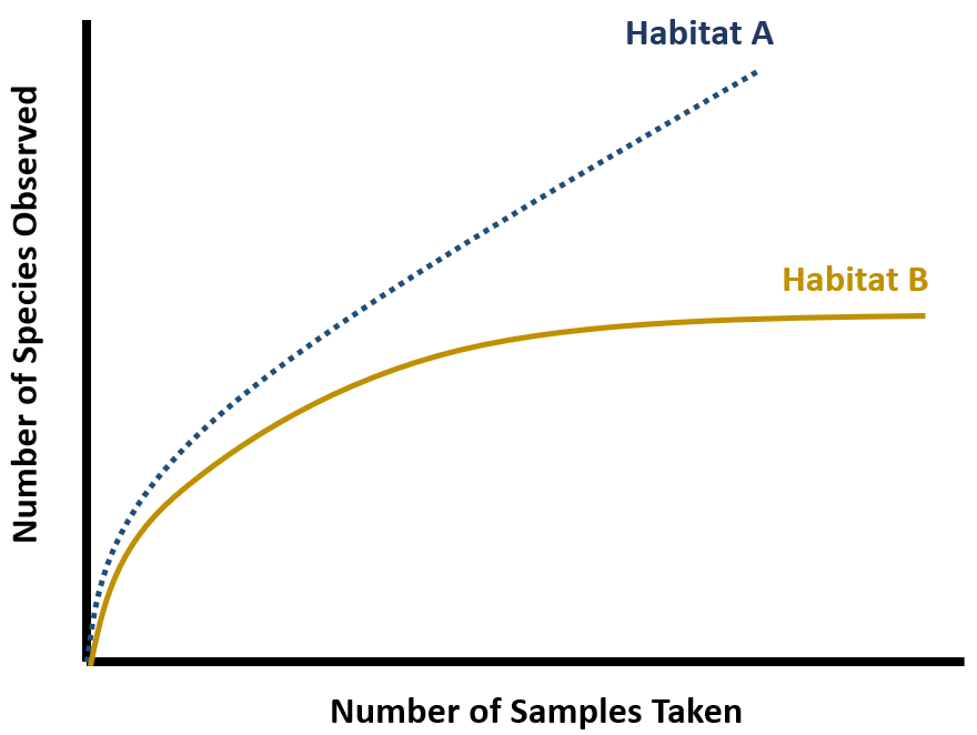
A simplified example of a rarefaction curve. In both habitats, the number of species observed (species richness) increases with the number of samples taken. In Habitat B, the curve eventually saturates (reaches an asymptote), suggesting that the actual species richness of the habitat has been reached. Habitat A, however, has not yet reached its asymptote, so additional sampling would reveal additional new species in this habitat. 

Case Study: The Deep Sea of the Mediterranean Basin 

From: Danovaro, R., Company, J.B., Corinaldesi, C., D'Onghia, G., Galil, B., Gambi, C., Gooday, A.J., Lampadariou, N., Luna, G.M., Morigi, C. and Olu, K., 2010. Deep-sea biodiversity in the Mediterranean Sea: the known, the unknown, and the unknowable. PloS one, 5(8), p.e11832.

Deep-sea ecosystems represent the largest biome of the global biosphere, but knowledge of their biodiversity is still scant. The Mediterranean basin has been proposed as a hotspot of terrestrial and coastal marine biodiversity, but has been supposed to be impoverished of deep-sea species richness. Danovaro et al. (2010) summarized all available information on benthic biodiversity (Prokaryotes, Foraminifera, Meiofauna, Macrofauna, and Megafauna) in different deep-sea ecosystems of the Mediterranean Sea (200 to more than 4,000 m depth), including open slopes, deep basins, canyons, cold seeps, seamounts, deep-water corals and deep-hypersaline anoxic basins and analyzed overall longitudinal and bathymetric patterns. 

 

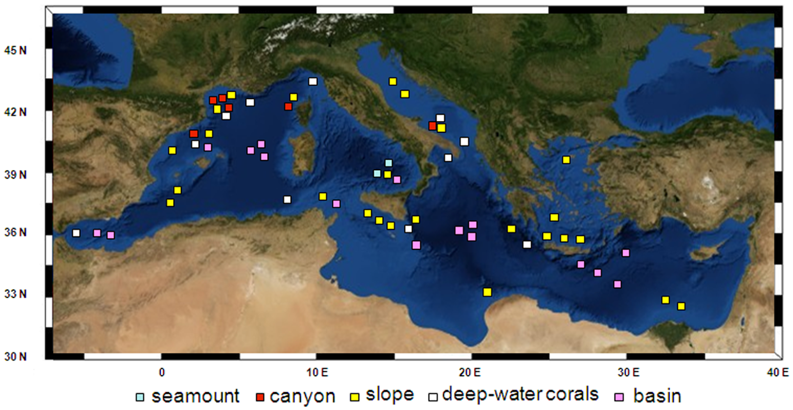
Figure 1. Investigated areas in the Mediterranean basin. Areas include slopes, seamounts, canyons, deep-water corals, and basin.

Danovaro et al. (2010) found that all of the biodiversity components, except Bacteria and Archaea, displayed a decreasing pattern with increasing water depth, but to a different extent for each component. Unlike patterns observed for faunal abundance, highest negative values of the slopes of the biodiversity patterns were observed for Meiofauna, followed by Macrofauna and Megafauna. Comparison of the biodiversity associated with open slopes, deep basins, canyons, and deep-water corals showed that the deep basins were the least diverse. Rarefaction curves allowed for estimation of the expected number of species for each benthic component in different bathymetric ranges. Species were unique across ecosystems, so each ecosystem contributes significantly to overall biodiversity. 

 

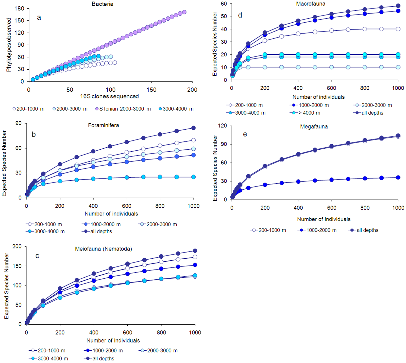
Figure 2. Rarefaction curves for the different components of the deep biota.

Danovaro et al. (2010) estimated that the overall deep-sea Mediterranean biodiversity (excluding prokaryotes) reaches approximately 2,805 species, of which about 66% is still undiscovered. Among the biotic components investigated (Prokaryotes excluded), most of the unknown species are within the phylum Nematoda, followed by Foraminifera, but an important fraction of macrofaunal and megafaunal species also remains unknown. The data in this study provide new insights into the patterns of biodiversity in the deep-sea Mediterranean and new clues for future investigations aimed at identifying the factors controlling and threatening deep-sea biodiversity.

Biodiversity at different scales- Alpha, Beta, and Gamma

Biologists have developed three quantitative measures of species diversity as a means of measuring and comparing species diversity:

• Alpha diversity (or species richness), the most commonly referenced measure of species diversity, refers to the total number of species found in a particular biological community, such as a lake or a forest. Bwindi Forest in Uganda, with an estimated 350 bird species, has one of the highest alpha diversities of all African ecosystems.

• Gamma diversity describes the total number of species that occur across an entire region, such as a mountain range or continent, that includes many ecosystems. The Albertine Rift, which includes Bwindi Forest, has more than 1,074 species of birds, a very high gamma diversity for such a small region.

• Beta diversity connects alpha and gamma diversity. It describes the rate at which species composition changes across a region. For example, if every wetland in a region was inhabited by a similar suite of plant species, then the region would have low beta diversity; in contrast, if several wetlands in a region had plants communities that were distinct and had little overlap with one another, the region would have high beta diversity. Beta diversity is calculated as gamma diversity divided by alpha diversity. The beta diversity for forest birds of the Albertine Rift is about 3.0, if each ecosystem in the area has about the same number of species as Bwindi Forest.

 

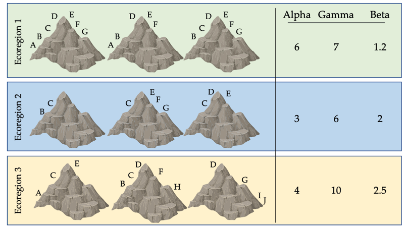
Figure \(\PageIndex{1}\): Biodiversity indices for nine mountain peaks across three ecoregions. Each symbol represents a different species; some species have populations on only one peak, while others are found on two or more peaks. The variation in species richness on each peak results in different alpha, gamma, and beta diversity values for each ecoregion. This variation has implications for how we divide limited resources to maximise protection. If only one ecoregion can be protected, ecoregion 3 may be a good choice because it has high gamma (total) diversity. However, if only one peak can be protected, should a peak in ecoregion 1 (with many widespread species) or ecoregion 3 (with several unique, range-restricted species) be protected? After Primack, 2012, CC BY 4.0.

It is important to note that alpha, beta, and gamma diversity describe only part of what is meant by biodiversity. For example, none of these three terms completely account for genetic diversity, which allows species to adapt as conditions change. It also neglects the importance of ecosystem diversity, which results from the collective response of species to their dynamic environment. However, these diversity measures are useful for comparing different regions, and identifying locations with high concentrations of native species that should be protected.

Functional Diversity and Indigenous Land Use Practices

Case Study Modified from Armstrong, C. G., Miller, J. E., McAlvay, A. C., Ritchie, P. M., & Lepofsky, D. (2021). Historical indigenous land-use explains plant functional trait diversity. Ecology and Society. 26: 6. This article was published under CC BY 4.0.

 

In addition to species diversity, ecologists are often interested in the trait or functional diversity of a community. A trait is simply any morphological, physiological or phenological feature measurable at the individual level (Reiss et al. 2009). Functional traits are those that define species in terms of their ecological roles - how they interact with the environment and with other species (Diaz and Cabido, 2001). 

Functional diversity is a biodiversity measure based on functional traits of the species present in a community. In ocean phytoplankton, for example, these traits usually include body size, tolerance and sensitivity to environmental conditions, motility, shape, and N-fixation ability (Reynolds et al., 2002; Weithoff G. 2003). In terrestrial plant communities, researchers have included more complex traits like rates of growth, nutrient requirements and water uptake (Walker and Langridge, 2002; Barnett et al, 2007). Functional traits are a critical tool for understanding ecological communities because they give insights into community assembly processes as well as potential species interactions and other ecosystem functions. Because there are a greater variety of “roles” being played in a system with higher functional diversity, this measure of diversity has often been linked to higher ecosystem productivity and stability.  

Human land-use legacies have long-term effects on plant community composition and ecosystem function and on the diversity of functional traits. Armstrong et al. (2021) studied how plant functional trait distributions and functional diversity are affected by ancient and historical Indigenous forest management in the Pacific Northwest. 

 

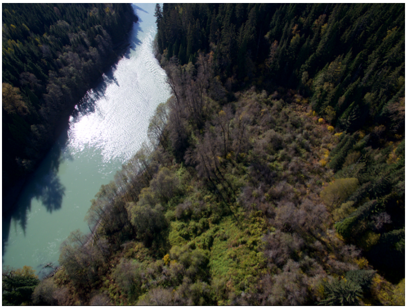
Figure \(\PageIndex{2}\): The Village complex of Dałk Gyilakyaw consists of three discrete villages and is the ancestral home of Gitsm’geelm (Ts’msyen) people. Note the dramatic vegetation change between the forest garden and encroaching conifers (“periphery forests”). Photograph: S. Carroll. 

 

Figure \(\PageIndex{3}\): Total Species Richness and Species Richness by Lifeform. Richness is indicated overall between forest gardens and periphery forests (averaged across the four of the study areas) and among the three growth forms (trees, shrubs and herbs)

 

For their research into plant functional diversity, Armstrong et al. (2021) compared forest garden ecosystems - managed perennial fruit and nut communities associated exclusively with archaeological village sites - with surrounding periphery conifer forests. To characterize the functional diversity of understory plant communities, they focused on four functional traits: seed mass, shade tolerance, pollination syndrome, and dispersal syndrome. These traits represent important axes of plant life-history variation and can also have important consequences for ecosystem functioning, while also having relevance to ethnobotanical plant uses (Pérez-Harguindeguy et al. 2013). For example, plants with animal-dispersed seeds may be able to disperse long distances and may also contribute to wildlife habitat by providing edible fruits; these plants are also more likely to be eaten by people.

 

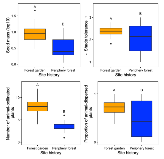
Figure \(\PageIndex{4}\): Functional Trait Measures between Forest Gardens and Periphery Forests. Comparisons of average seed mass, shade tolerance, pollination syndrome, and dispersal syndrome traits for herbs and shrubs across forest gardens and peripheral forests — all are significantly higher in the forest gardens.

 

Armstrong et al. (2021) found that forest gardens have substantially greater plant and functional trait diversity than periphery forests, even more than 150 years after management ceased. Forests managed by Indigenous peoples in the past now provide diverse resources and habitat for animals and other pollinators and are more rich than naturally forested ecosystems. Although ecological studies rarely incorporate Indigenous land-use legacies, the positive effects of Indigenous land use on contemporary functional and taxonomic diversity found by Armstrong et al. (2021) suggest that Indigenous management practices are tied to ecosystem health and resilience.

 

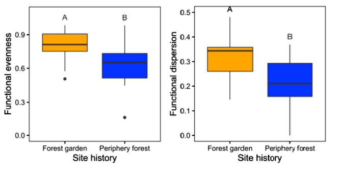
Figure \(\PageIndex{5}\): Functional Diversity Measures between Forest Gardens and Periphery Forests. Functional evenness (the evenness of functional trait distribution in niche space; Villéger et al. 2008) and functional dispersion (the average distance to the abundance-weighted centroid of functional trait values; Laliberté, and Legendre 2010) were significantly greater in forest gardens as compared to periphery forests. Comparisons of functional diversity at forest gardens and peripheral forests. 

Sources

Pielou, E.C. (1966). The measurement of diversity in different types of biological collections. Journal of Theoretical Biology. 13: 131–144. doi:10.1016/0022-5193(66)90013-0.

Simpson, E.H. (1949) Measurement of diversity. Nature, 163, 688. doi:10.1038/163688a0

Shannon, C.E. (1948) A Mathematical Theory of Communication. The Bell System Technical Journal, 27, 379-423.
https://doi.org/10.1002/j.1538-7305.1948.tb01338.x

 

Attributions

Section written and curated by A. Wilson and N. Gownaris, with material from the following open-access resources: 

• Conservation Biology in Sub-Saharan Africa by John W. Wilson and Richard B. Primack
• Diversity Index by Wikipedia, the free Encyclopedia