8.10: Sanger Sequencing of DNA

Radioactive Chain Termination

The polymerization of nucleic acids occurs in a 5′ → 3′ direction. The 5′ position has a phosphate group while the 3′ position of the hexose has a hydroxyl group. Polymerization depends on these 2 functional groups in order for a dehydration synthesis reaction to occur and extend the sugar-phosphate backbone of the nucleic acid. In the 1970s, Fred Sanger’s group discovered a fundamentally new method of ‘reading’ the linear DNA sequence using special bases called chain terminators or dideoxynucleotides. The absence of a hydroxyl group at the 3′ position blocks the polymerization, resulting in termination. This method is still in use today and is called "Sanger dideoxynucleotide chain-termination method". This method originally used a radioactively labeled primer to initiate the sequencing reaction. Four reactions take place where each reaction is intentionally “poisoned” with a dideoxy chain terminator. For example, one reaction will have all 4 dNTPs (deoxynucleotide triphosphates) with the addition to a small amount of ddATP (dideoxyadenosine triphosphate). This reaction will result in a series of premature terminations of the polymerization specifically at different locations where an Adenine would be incorporated.

dATP is a natural monomer used in the polymerization of DNA. The 3′-OH is the attachment point of the next subsequent nucleotide.

The lack of a 3′-OH in this molecule of ddATP makes it a chain terminator that will prohibit the addition of another nucleotide to the DNA polymer.

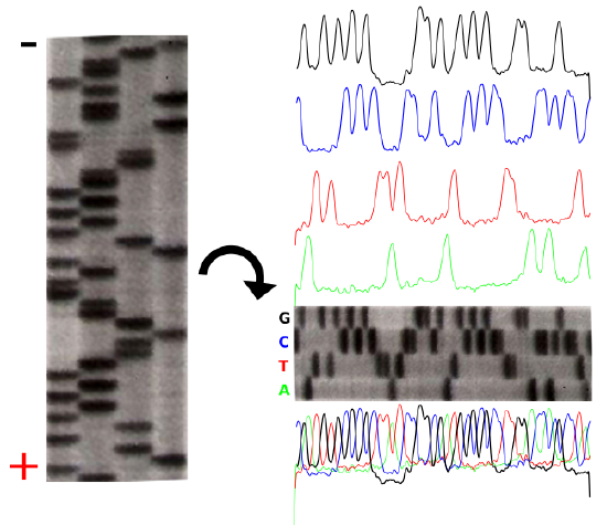
The product of these 4 separate sequencing reactions is run on a large polyacrylamide sequencing gels. The smallest fragments run through the gel the fastest and create a ladder-like pattern. This can be visualized through the use of an x-ray film that is sensitive to the radioactivity. Each lane of the gel corresponds to one of the four chain-terminating reactions. The bases are read sequentially from the bottom up and reveal the sequence of the DNA.

The sequencing gel can be manually scored. The profiles of each lane have been created using ImageJ to illustrate the banding pattern and subsequent sequence.

Credit: John Schmidt & Jeremy Seto (CC-BY-SA 3.0)

Fluorescent Chain Termination and Capillary Electrophoresis

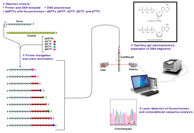
Credit: Estevezj (CC-BY-SA 3.0)

Radioactivity is dangerous and undesirable to work with so chain terminators with fluorescent tags were developed. This method synthesizes a series of DNA strands that are specifically fluorescent at the termination that is passed through a capillary electrophoresis system. As the fragments of DNA pass a laser and detector, the different fluorescent signal attributed to each ddNTP is identified and generates a chromatogram to represent the sequence. Fluorescent Chain Terminators are now used in reactions and run through a small capillary. The smallest fragments run through first and are detected to reveal a chromatogram.

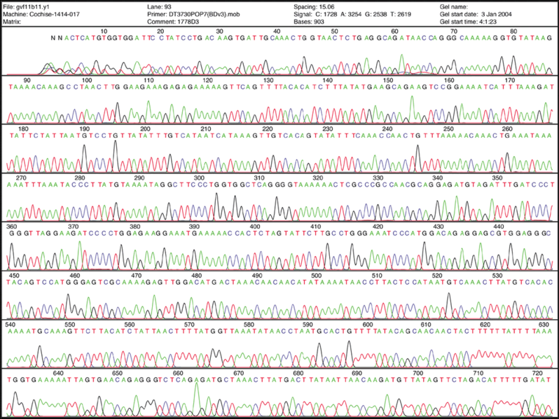
Fluorescent Chromatograms are used to score the nucleotide chain termination. The amplitude of each peak corresponds to the strength or certainty of the nucleotide call. Chromatogram files are usually provided alongside the sequence file with the extension *.ab1 while the sequence files are provided as a text file in the fasta format. More about these files can be found here. The ab1 files are extremely important to analyze when there are ambiguity or sequencing errors. These ab1 files can also be used to ascribe a quality score on the base call.

When there is too much ambiguity in the signal because of multiple peaks, you will often find an N in place of one of the 4 nucleotides (A, T, C, and G).

This video (source: www.yourgenome.org CC-BY) illustrates the mechanism of fluorescent chain termination and capillary electrophoresis.

Sequencing Genomes

Credit: Jeremy Seto (CC-BY-NC-SA 3.0)

Traditional sequencing of genomes was a long and tedious process that cloned fragments of genomic DNA into plasmids to generate a genomic DNA library (gDNA). These plasmids were individually sequenced using Sanger sequencing methodology and computational was performed to identify overlapping pieces, like a jigsaw puzzle. This assembly would result in a draft scaffold.

The video below is taken from yourgenome.org (CC-BY) and illustrates the sequencing of the human genome through the shotgun sequencing approach.