6.3: Oceanic Circulation

Not unexpectedly, the oceans are warmest near the equator—typically 25° to 30°C—and coldest near the poles—around 0°C (Figure \(\PageIndex{7}\)). (Sea water will remain unfrozen down to about -2°C) Variations in sea-surface temperatures (SST) are related to redistribution of water by ocean currents, as we will see below. A good example of that is the plume of warm Gulf Stream water that extends across the northern Atlantic. St. John’s, Newfoundland, and Brittany in France are at about the same latitude (47.5° N), but the average SST in St. John’s is a frigid 3°C, while that in Brittany is a reasonably comfortable 15°C.

Figure \(\PageIndex{7}\): The global distribution of average annual sea-surface temperatures.
Source: Plumbago, licensed under CC BY-SA.

Currents in the open ocean are created by wind moving across the water and by density differences related to temperature and salinity. An overview of the main ocean currents is shown in Figure \(\PageIndex{8}\). As you can see, the northern hemisphere currents form circular patterns (gyres) that rotate clockwise, while the southern hemisphere gyres are counter-clockwise. This happens for the same reason that the water in your northern hemisphere sink rotates in a clockwise direction as it flows down the drain; this is caused by the Coriolis effect.

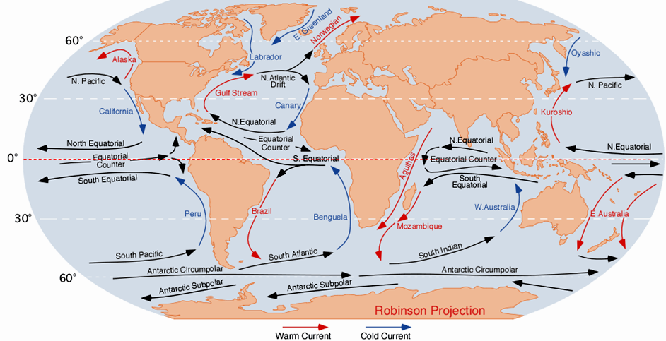
Figure \(\PageIndex{8}\): Overview of the main open-ocean currents. Red arrows represent warm water moving toward colder regions. Blue arrows represent cold water moving toward warmer regions. Black arrows represent currents that don’t involve significant temperature changes.
Source: image “Corrientes Oceanicas” by Dr. Michael Pidwirny is available in the public domain.

Because the ocean basins are not like bathroom basins, not all ocean currents behave the way we would expect. In the North Pacific, for example, the main current flows clockwise, but there is a secondary current in the area adjacent to our coast—the Alaska Current—that flows counter-clockwise, bringing relatively warm water from California, past Oregon, Washington, and B.C. to Alaska. On Canada’s eastern coast, the cold Labrador Current flows south past Newfoundland, bringing a stream of icebergs past the harbour at St. John’s (Figure \(\PageIndex{9}\)). This current helps to deflect the Gulf Stream toward the northeast, ensuring that Newfoundland stays cool, and western Europe stays warm.

Figure \(\PageIndex{9}\): An iceberg floating past Exploits Island on the Labrador Current.
Source: image “Newfoundland Iceberg” by Shawn is licensed under CC BY-SA 2.0.

The currents shown in Figure \(\PageIndex{8}\) are all surface currents, and they only involve the upper few hundred meters of the oceans. But there is much more going on underneath. The Gulf Stream, for example, which is warm and saline, flows past Britain and Iceland into the Norwegian Sea (where it becomes the Norwegian Current). As it cools down, it becomes denser, and because of its high salinity, which also contributes to its density, it starts to sink beneath the surrounding water (Figure \(\PageIndex{10}\)). At this point, it is known as North Atlantic Deep Water (NADW), and it flows to significant depth in the Atlantic as it heads back south. Meanwhile, at the southern extreme of the Atlantic, very cold water adjacent to Antarctica also sinks to the bottom to become Antarctic Bottom Water (AABW) which flows to the north, underneath the NADW.

Figure \(\PageIndex{10}\): A depiction of the vertical movement of water along a north-south cross-section through the Atlantic basin.
Source: Steven Earle, licensed under CC BY.

The descent of the dense NADW is just one part of a global system of seawater circulation, both at surface and at depth, as illustrated in Figure \(\PageIndex{11}\)). The water that sinks in the areas of deep water formation in the Norwegian Sea and adjacent to Antarctica moves very slowly at depth. It eventually resurfaces in the Indian Ocean between Africa and India, and in the Pacific Ocean, north of the equator.

Figure \(\PageIndex{11}\): The thermohaline circulation system, also known as the Global Ocean Conveyor. Source: image "A summary of the path of thermohaline circulation" by NASA is available in the public domain.

The thermohaline circulation is critically important to the transfer of heat on Earth. It brings warm water from the tropics to the poles, and cold water from the poles to the tropics, thus keeping polar regions from getting too cold and tropical regions from getting too hot. A reduction in the rate of thermohaline circulation would lead to colder conditions and enhanced formation of sea ice at the poles. This would start a positive feedback process that could result in significant global cooling. There is compelling evidence to indicate that there were major changes in thermohaline circulation, corresponding with climate changes, during the Pleistocene Glaciation.

The movement of surface currents also plays a role in the vertical movements of deeper water, mixing the upper water column. Upwelling is the process that brings deeper water to the surface, and its major significance is that it brings nutrient-rich deep water to the nutrient-deprived surface, stimulating primary production (see section 7.3). Downwelling is where surface water is forced downwards, where it may deliver oxygen to deeper water. Downwelling leads to reduced productivity, as it extends the depth of the nutrient-limited layer. For more details on upwelling, downwelling, and ocean productivity see the section of Dr. Paul Webb's Oceanography book on Currents, Upwelling and Downwelling.  

There are several interactions between ocean currents, ocean temperatures, and atmospheric circulation that cause cyclic global climate variability.  The most well know of which is the El Niño/Southern Oscillation (ENSO) in the Pacific Ocean [also called El Niño-La Niña Cycles] associated with a band of warm ocean water that develops in the central and east-central equatorial Pacific. For more information on El Niño and La Niña, see the section of Dr. Paul Webb's Oceanography book on El Niño and La Niña.  El Niño/Southern Oscillation (ENSO) is perhaps the most important ocean-atmosphere interaction phenomenon to cause cyclic global climate variability. 

 

Contributors and Attributions

This page was modified from the following sources by Kyle Whittinghill (University of Vermont)

• 18.4 Ocean Water from Physical Geology by Steven Earle (licensed under CC-BY)
• 8.2 Winds and the Coriolis Effect from Introduction to Oceanography by Paul Webb (licensed under CC-BY)
• 8.3 Winds and Climate from Introduction to Oceanography by Paul Webb (licensed under CC-BY)
• 9.5: Currents, Upwelling and Downwelling from Introduction to Oceanography by Paul Webb (licensed under CC-BY)
• 9.6: El Niño and La Niña from Introduction to Oceanography by Paul Webb (licensed under CC-BY)
• 10.02: Controls of Climate from Physical Geography and Natural Disasters by Adam Dastrup (licensed under CC BY-NC-SA 4.0)