4.2.2: Dihybrid Crosses and Independent Assortment

Mendel’s Second Law

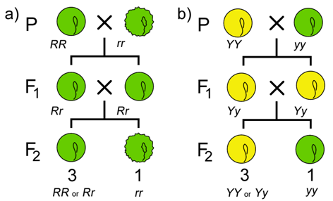
Before Mendel, it had not yet been established that heritable traits were controlled by discrete factors. Therefore an important question was whether distinct traits were controlled by separate factors that were inherited independently of one another. To answer this, Mendel took two apparently unrelated traits, such as seed shape and seed color, and studied their inheritance together in one individual. He studied two variants of each trait: seed color was either green or yellow, and seed shape was either round or wrinkled. When either of these traits was studied individually, the phenotypes segregated in the classical 3:1 ratio among the progeny of a monohybrid cross, with ¾ of the seeds green and ¼ yellow in one cross, and ¾ round and ¼ wrinkled in the other cross. Would this be true when both were in the same individual?

Figure \(\PageIndex{1}\): Monohybrid crosses involving two distinct traits, shape which can be round or wrinkled and color which can be yellow or green. a) A monohybrid cross between RR (round peas) and rr (wrinkled peas) plants and b) A monohybrid cross between YY (yellow peas) and yy (green peas) plants. (Original-Deyholos-CC:AN)

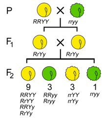
To analyze the segregation of both traits at the same time in the same individual, Mendel crossed a pure breeding line of green, wrinkled peas with a pure breeding line of yellow, round peas to produce F₁ progeny that were all yellow and round, and which were also dihybrids; they carried two alleles at each of two loci. If the alleles for the two genes for pea shape and pea color cannot be separated from each other, then in the F₂ generation, the offspring should be only green, round pea plants or yellow, wrinkled plants, like the P generation plants.

If the genes controlling shape and color can be inherited independently, then what is the probability of phenotypes in the F₂ generation? Using the product rule, we can multiply the individual probabilities of obtaining a round phenotype (¾) with the probability of obtaining a yellow phenotype (¾), then ¾ × ¾ = 9/16 of the progeny would be both round and green. Likewise, ¾ × ¼ = 3/16 of the progeny would be both round and yellow, and so on. By applying the product rule to all combinations of phenotypes, we can predict a 9:3:3:1 phenotypic ratio among the progeny of a dihybrid cross, if certain conditions are met, including the independent segregation of the alleles at each locus.

Definition: Product Rule

The probability of two or more independent events occurring is the product obtained by multiplying the probabilities of the individual events. If you can use the word "and" to describe the occurrence of the events, then you can usually use the product rule.

For example, the probability of an organism with phenotype 1 and phenotype 2 is the product of the probability of phenotype 1 times the probability of phenotype 2.

The dihybrid crosses that Mendel performed consistently revealed the 9:3:3:1 ratio in dihybrid crosses, leading him to conclude that the factors controlling the traits are inherited independent of one another, a rule commonly known as the Law of Independent Assortment. Importantly, the F₂ generation includes two phenotype classes (in this example, round, green peas and yellow, wrinkled peas) that are new combinations of phenotypes, distinct from the parental generation plants. Thus, independent assortment contribute to genetic diversity.

Figure \(\PageIndex{2}\): Pure-breeding lines RRYY and rryy are crossed to produce dihybrids in the F₁ generation. The cross of the F₁ RrYy dihybrids produces four phenotypic classes in a ratio of 9:3:3:1. (Original-Deyholos-CC:AN)

Definition: Mendel's Second Law

The Law of Independent Assortment states that two loci assort independently of each other during gamete formation.

Table \(\PageIndex{1}\): Phenotypic classes expected in monohybrid and dihybrid crosses for two seed traits in pea.

						Frequency of phenotypic crosses within separate monohybrid crosses: seed shape: ¾ round ¼ wrinkled seed color: ¾ yellow ¼ green Frequency of phenotypic crosses within a dihybrid cross: ¾ round × ¾ yellow = 9/16 round & yellow ¾ round × ¼ green = 3/16 round & green ¼ wrinkled × ¾ yellow = 3/16 wrinkled & yellow ¼ wrinkled × ¼ green = 1/16 wrinkled & green

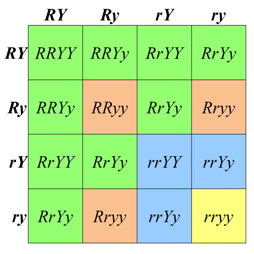
The 9:3:3:1 phenotypic ratio calculated using the product rule can also be obtained using Punnett Square. First, we list the genotypes of the possible gametes along each axis of the Punnett Square. In a diploid with two heterozygous genes of interest, there are up to four combinations of alleles in the gametes of each parent. The gametes from the respective rows and column are then combined in the each cell of the array. When working with two loci, genotypes are written with the symbols for both alleles of one locus, followed by both alleles of the next locus (e.g. AaBb, not ABab). Note that the order in which the loci are written does not imply anything about the actual position of the loci on the chromosomes.

Figure \(\PageIndex{3}\): A Punnett Square showing the results of a dihybrid cross. Each of the four phenotypic classes is represented by a different color of shading. (Original-Deyholos-CC:AN)

 

To calculate the expected phenotypic ratios, we assign a phenotype to each of the 16 genotypes in the Punnett Square, based on our knowledge of the alleles and their dominance relationships. In the case of Mendel’s seeds, any genotype with at least one R allele and one Y allele will be round and yellow; these genotypes are shown in the nine, green-shaded cells. We can represent all of four of the different genotypes shown in these cells with the notation (R_Y_), where the blank line (__), means “any allele”. The three offspring that have at least one R allele and are homozygous recessive for y (i.e. R_yy) will have a round, green phenotype. Conversely the three progeny that are homozygous recessive r, but have at least one Y allele (rrY_) will have wrinkled, yellow seeds. Finally, the rarest phenotypic class of wrinkled, yellow seeds is produced by the doubly homozygous recessive genotype, rryy, which is expected to occur in only one of the sixteen possible offspring represented in the square.

 

Video \(\PageIndex{1}\): Watch the video to see how to set up and complete a dihybrid Punnett Square.

Assumptions of the 9:3:3:1 ratio

Both the product rule and the Punnett Square approaches showed that a 9:3:3:1 phenotypic ratio is expected among the progeny of a dihybrid cross such as Mendel’s RrYy × RrYy. In making these calculations, we assumed that:

1. both loci assort independently;
2. one allele at each locus is completely dominant; and
3. each of four possible phenotypes can be distinguished unambiguously, with no interactions between the two genes that would alter the phenotypes.

Deviations from the 9:3:3:1 phenotypic ratio may indicate that one or more of the above conditions has not been met. Modified ratios in the progeny of a dihybrid cross can therefore reveal useful information about the genes involved.

Query \(\PageIndex{1}\)

Applying the product rule

Mendel's conclusions about the segregation of alleles and independent of assortment of genes continue to hold true for inheritance in diploid organisms, in which meiosis produces gametes that have one copy of thousands genes - not just one or two. However, making a Punnett Square for more than two genes becomes tricky and cumbersome. The Product Rule can be used to predict outcomes when considering more than two genes at a time. Find the probability of each genotype or phenotype and multiple each probability.

Exercise \(\PageIndex{1}\)

If two organisms with genotype GgHhJi are crossed, what percent of offspring are expected to be homozygous dominant for all three genes?

Hint: GG and HH and JJ

Answer

(Probability GG: 1/4) x (Probability HH: 1/4) x (Probability JJ: 1/4) = 1/64

Contributors and Attributions

• Dr. Todd Nickle and Isabelle Barrette-Ng (Mount Royal University) The content on this page is licensed under CC SA 3.0 licensing guidelines.

• Stefanie Leacock, UA-Little Rock