Biology LibreTexts

2.2.4: B4. Analysis of Protein Secondary Structure

  • Page ID
    64210
  • \( \newcommand{\vecs}[1]{\overset { \scriptstyle \rightharpoonup} {\mathbf{#1}} } \)

    \( \newcommand{\vecd}[1]{\overset{-\!-\!\rightharpoonup}{\vphantom{a}\smash {#1}}} \)

    \( \newcommand{\id}{\mathrm{id}}\) \( \newcommand{\Span}{\mathrm{span}}\)

    ( \newcommand{\kernel}{\mathrm{null}\,}\) \( \newcommand{\range}{\mathrm{range}\,}\)

    \( \newcommand{\RealPart}{\mathrm{Re}}\) \( \newcommand{\ImaginaryPart}{\mathrm{Im}}\)

    \( \newcommand{\Argument}{\mathrm{Arg}}\) \( \newcommand{\norm}[1]{\| #1 \|}\)

    \( \newcommand{\inner}[2]{\langle #1, #2 \rangle}\)

    \( \newcommand{\Span}{\mathrm{span}}\)

    \( \newcommand{\id}{\mathrm{id}}\)

    \( \newcommand{\Span}{\mathrm{span}}\)

    \( \newcommand{\kernel}{\mathrm{null}\,}\)

    \( \newcommand{\range}{\mathrm{range}\,}\)

    \( \newcommand{\RealPart}{\mathrm{Re}}\)

    \( \newcommand{\ImaginaryPart}{\mathrm{Im}}\)

    \( \newcommand{\Argument}{\mathrm{Arg}}\)

    \( \newcommand{\norm}[1]{\| #1 \|}\)

    \( \newcommand{\inner}[2]{\langle #1, #2 \rangle}\)

    \( \newcommand{\Span}{\mathrm{span}}\) \( \newcommand{\AA}{\unicode[.8,0]{x212B}}\)

    \( \newcommand{\vectorA}[1]{\vec{#1}}      % arrow\)

    \( \newcommand{\vectorAt}[1]{\vec{\text{#1}}}      % arrow\)

    \( \newcommand{\vectorB}[1]{\overset { \scriptstyle \rightharpoonup} {\mathbf{#1}} } \)

    \( \newcommand{\vectorC}[1]{\textbf{#1}} \)

    \( \newcommand{\vectorD}[1]{\overrightarrow{#1}} \)

    \( \newcommand{\vectorDt}[1]{\overrightarrow{\text{#1}}} \)

    \( \newcommand{\vectE}[1]{\overset{-\!-\!\rightharpoonup}{\vphantom{a}\smash{\mathbf {#1}}}} \)

    \( \newcommand{\vecs}[1]{\overset { \scriptstyle \rightharpoonup} {\mathbf{#1}} } \)

    \( \newcommand{\vecd}[1]{\overset{-\!-\!\rightharpoonup}{\vphantom{a}\smash {#1}}} \)

    \(\newcommand{\avec}{\mathbf a}\) \(\newcommand{\bvec}{\mathbf b}\) \(\newcommand{\cvec}{\mathbf c}\) \(\newcommand{\dvec}{\mathbf d}\) \(\newcommand{\dtil}{\widetilde{\mathbf d}}\) \(\newcommand{\evec}{\mathbf e}\) \(\newcommand{\fvec}{\mathbf f}\) \(\newcommand{\nvec}{\mathbf n}\) \(\newcommand{\pvec}{\mathbf p}\) \(\newcommand{\qvec}{\mathbf q}\) \(\newcommand{\svec}{\mathbf s}\) \(\newcommand{\tvec}{\mathbf t}\) \(\newcommand{\uvec}{\mathbf u}\) \(\newcommand{\vvec}{\mathbf v}\) \(\newcommand{\wvec}{\mathbf w}\) \(\newcommand{\xvec}{\mathbf x}\) \(\newcommand{\yvec}{\mathbf y}\) \(\newcommand{\zvec}{\mathbf z}\) \(\newcommand{\rvec}{\mathbf r}\) \(\newcommand{\mvec}{\mathbf m}\) \(\newcommand{\zerovec}{\mathbf 0}\) \(\newcommand{\onevec}{\mathbf 1}\) \(\newcommand{\real}{\mathbb R}\) \(\newcommand{\twovec}[2]{\left[\begin{array}{r}#1 \\ #2 \end{array}\right]}\) \(\newcommand{\ctwovec}[2]{\left[\begin{array}{c}#1 \\ #2 \end{array}\right]}\) \(\newcommand{\threevec}[3]{\left[\begin{array}{r}#1 \\ #2 \\ #3 \end{array}\right]}\) \(\newcommand{\cthreevec}[3]{\left[\begin{array}{c}#1 \\ #2 \\ #3 \end{array}\right]}\) \(\newcommand{\fourvec}[4]{\left[\begin{array}{r}#1 \\ #2 \\ #3 \\ #4 \end{array}\right]}\) \(\newcommand{\cfourvec}[4]{\left[\begin{array}{c}#1 \\ #2 \\ #3 \\ #4 \end{array}\right]}\) \(\newcommand{\fivevec}[5]{\left[\begin{array}{r}#1 \\ #2 \\ #3 \\ #4 \\ #5 \\ \end{array}\right]}\) \(\newcommand{\cfivevec}[5]{\left[\begin{array}{c}#1 \\ #2 \\ #3 \\ #4 \\ #5 \\ \end{array}\right]}\) \(\newcommand{\mattwo}[4]{\left[\begin{array}{rr}#1 \amp #2 \\ #3 \amp #4 \\ \end{array}\right]}\) \(\newcommand{\laspan}[1]{\text{Span}\{#1\}}\) \(\newcommand{\bcal}{\cal B}\) \(\newcommand{\ccal}{\cal C}\) \(\newcommand{\scal}{\cal S}\) \(\newcommand{\wcal}{\cal W}\) \(\newcommand{\ecal}{\cal E}\) \(\newcommand{\coords}[2]{\left\{#1\right\}_{#2}}\) \(\newcommand{\gray}[1]{\color{gray}{#1}}\) \(\newcommand{\lgray}[1]{\color{lightgray}{#1}}\) \(\newcommand{\rank}{\operatorname{rank}}\) \(\newcommand{\row}{\text{Row}}\) \(\newcommand{\col}{\text{Col}}\) \(\renewcommand{\row}{\text{Row}}\) \(\newcommand{\nul}{\text{Nul}}\) \(\newcommand{\var}{\text{Var}}\) \(\newcommand{\corr}{\text{corr}}\) \(\newcommand{\len}[1]{\left|#1\right|}\) \(\newcommand{\bbar}{\overline{\bvec}}\) \(\newcommand{\bhat}{\widehat{\bvec}}\) \(\newcommand{\bperp}{\bvec^\perp}\) \(\newcommand{\xhat}{\widehat{\xvec}}\) \(\newcommand{\vhat}{\widehat{\vvec}}\) \(\newcommand{\uhat}{\widehat{\uvec}}\) \(\newcommand{\what}{\widehat{\wvec}}\) \(\newcommand{\Sighat}{\widehat{\Sigma}}\) \(\newcommand{\lt}{<}\) \(\newcommand{\gt}{>}\) \(\newcommand{\amp}{&}\) \(\definecolor{fillinmathshade}{gray}{0.9}\)

    The percent and type of secondary structure can be determined using circular dichroism (CD) spectroscopy. (The links below come from an animated tutorial on Electromagnetic Waves and Circular Dichroism by András Szilágyi ) In this method, right and left circularly polarized light illuminates a protein, which, since it is made of all L-amino acids, is chiral. (The mirror image would be a protein of the same sequence made of D-amino acids.) Circularly polarized light can be made when plane polarized light of the same amplitude and wavelength meet out of phase. If R and L circularly polarized light of the same wavelength and amplitude are passed through an optically inactive medium, the two waves combine (vectorially) to produce plane polarized light. Optical activity is observed only when the environment in which a transition occurs is asymmetric.

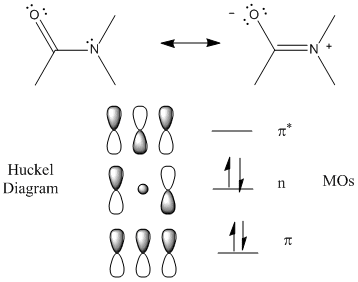
    The peptide (amide) bond absorbs UV light in the range of 180 to 230 nm (far-UV range) so this region of the spectra give information about the protein backbone, and more specifically, the secondary structure of the protein. The main transitions are n --> p* at 220 nm and p --> p* at 190 nm. There is a little contribution from aromatic amino acid side chains but it is small given the large number of peptide bonds. The lone pair on N adjacent to the pi bond can be considered to be rehybrized to sp2 from sp3 allowing for conjugation of the p electrons (which lowers the energy of the electrons). The Huckel diagram below shows 3 MOs generated form the 3 atomic p orbitals. The middle one (with 1 node) has energy similar to the separate atomic p orbtials and is considered a nonbonding MO (consistent with the lone nonbonding pair on the N atom).

    Figure: Peptide Bonds - MOs and Huckel Diagram
    PepBondMOsHuckel.gif

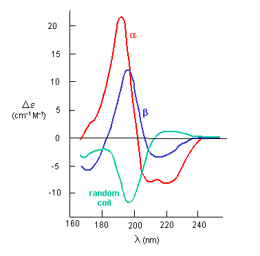
    The peptide bonds in a protein's asymmetric environment will absorb this range of light (promoting electrons to higher energy levels). In different secondary structures , the peptide bond electrons will absorb right and left circularly polarized light differently (for example, they have different molar absorptivities). Hence a, b and random coil structures all have distinguishable far UV CD spectra.

    Stated in another way, if plane polarized light, which is a superposition of right and left circularly polarized light, passes through an asymmetric sample which absorbs right and left circularly polarized differently (i.e they display circular dichroism), then the light passing through the sample after vector addition of the right and left hand circularly polarized light gives elliptically polarized light. (Great link!) The

    If the chiral molecules also have a different index of refraction for R and L circularly polarized light, an added net effect is rotation of the angle of the ellipitically of the polarized light. The far-UV CD spectrum of the protein is sensitive to the main chain conformation. The CD spectra of alpha and beta secondary structure are shown in the figure below.

    Figure: The CD Spectra of Alpha-Helix, Beta-Sheet, and Random Coils
    cdsecondst.gif

    Protein side chains also find themselves in such an asymmetric environment. If irradiated with circularly polarized UV light in the range of 250-300 nm (near UV), differential absorption of right and circularly polarized light by the aromatic amino acids (Tyr, Phe, Trp) and disulfide bonds occur and a near UV CD spectra result. If the near UV CD spectra of a protein is taken under two different sets of conditions, and the spectra differ, then it can be surmised that the environment of the side chains is different, and hence the proteins have somewhat different conformations. It will not give information about secondary structure of the backbone since that requires lower wavelengths for absorption of occur. Rather it can show differences in tertiary structure.

    • iconexternal_link.gifCD Spectroscopy - web tutorial

    This page titled 2.2.4: B4. Analysis of Protein Secondary Structure is shared under a CC BY-NC-SA license and was authored, remixed, and/or curated by Henry Jakubowski.

    • Was this article helpful?