
3.2: Total Magnification, Calculating Field of View, and Estimating Specimen Size
- Page ID
- 159069
\( \newcommand{\vecs}[1]{\overset { \scriptstyle \rightharpoonup} {\mathbf{#1}} } \)
\( \newcommand{\vecd}[1]{\overset{-\!-\!\rightharpoonup}{\vphantom{a}\smash {#1}}} \)
\( \newcommand{\dsum}{\displaystyle\sum\limits} \)
\( \newcommand{\dint}{\displaystyle\int\limits} \)
\( \newcommand{\dlim}{\displaystyle\lim\limits} \)
\( \newcommand{\id}{\mathrm{id}}\) \( \newcommand{\Span}{\mathrm{span}}\)
( \newcommand{\kernel}{\mathrm{null}\,}\) \( \newcommand{\range}{\mathrm{range}\,}\)
\( \newcommand{\RealPart}{\mathrm{Re}}\) \( \newcommand{\ImaginaryPart}{\mathrm{Im}}\)
\( \newcommand{\Argument}{\mathrm{Arg}}\) \( \newcommand{\norm}[1]{\| #1 \|}\)
\( \newcommand{\inner}[2]{\langle #1, #2 \rangle}\)
\( \newcommand{\Span}{\mathrm{span}}\)
\( \newcommand{\id}{\mathrm{id}}\)
\( \newcommand{\Span}{\mathrm{span}}\)
\( \newcommand{\kernel}{\mathrm{null}\,}\)
\( \newcommand{\range}{\mathrm{range}\,}\)
\( \newcommand{\RealPart}{\mathrm{Re}}\)
\( \newcommand{\ImaginaryPart}{\mathrm{Im}}\)
\( \newcommand{\Argument}{\mathrm{Arg}}\)
\( \newcommand{\norm}[1]{\| #1 \|}\)
\( \newcommand{\inner}[2]{\langle #1, #2 \rangle}\)
\( \newcommand{\Span}{\mathrm{span}}\) \( \newcommand{\AA}{\unicode[.8,0]{x212B}}\)
\( \newcommand{\vectorA}[1]{\vec{#1}} % arrow\)
\( \newcommand{\vectorAt}[1]{\vec{\text{#1}}} % arrow\)
\( \newcommand{\vectorB}[1]{\overset { \scriptstyle \rightharpoonup} {\mathbf{#1}} } \)
\( \newcommand{\vectorC}[1]{\textbf{#1}} \)
\( \newcommand{\vectorD}[1]{\overrightarrow{#1}} \)
\( \newcommand{\vectorDt}[1]{\overrightarrow{\text{#1}}} \)
\( \newcommand{\vectE}[1]{\overset{-\!-\!\rightharpoonup}{\vphantom{a}\smash{\mathbf {#1}}}} \)
\( \newcommand{\vecs}[1]{\overset { \scriptstyle \rightharpoonup} {\mathbf{#1}} } \)
\(\newcommand{\longvect}{\overrightarrow}\)
\( \newcommand{\vecd}[1]{\overset{-\!-\!\rightharpoonup}{\vphantom{a}\smash {#1}}} \)
\(\newcommand{\avec}{\mathbf a}\) \(\newcommand{\bvec}{\mathbf b}\) \(\newcommand{\cvec}{\mathbf c}\) \(\newcommand{\dvec}{\mathbf d}\) \(\newcommand{\dtil}{\widetilde{\mathbf d}}\) \(\newcommand{\evec}{\mathbf e}\) \(\newcommand{\fvec}{\mathbf f}\) \(\newcommand{\nvec}{\mathbf n}\) \(\newcommand{\pvec}{\mathbf p}\) \(\newcommand{\qvec}{\mathbf q}\) \(\newcommand{\svec}{\mathbf s}\) \(\newcommand{\tvec}{\mathbf t}\) \(\newcommand{\uvec}{\mathbf u}\) \(\newcommand{\vvec}{\mathbf v}\) \(\newcommand{\wvec}{\mathbf w}\) \(\newcommand{\xvec}{\mathbf x}\) \(\newcommand{\yvec}{\mathbf y}\) \(\newcommand{\zvec}{\mathbf z}\) \(\newcommand{\rvec}{\mathbf r}\) \(\newcommand{\mvec}{\mathbf m}\) \(\newcommand{\zerovec}{\mathbf 0}\) \(\newcommand{\onevec}{\mathbf 1}\) \(\newcommand{\real}{\mathbb R}\) \(\newcommand{\twovec}[2]{\left[\begin{array}{r}#1 \\ #2 \end{array}\right]}\) \(\newcommand{\ctwovec}[2]{\left[\begin{array}{c}#1 \\ #2 \end{array}\right]}\) \(\newcommand{\threevec}[3]{\left[\begin{array}{r}#1 \\ #2 \\ #3 \end{array}\right]}\) \(\newcommand{\cthreevec}[3]{\left[\begin{array}{c}#1 \\ #2 \\ #3 \end{array}\right]}\) \(\newcommand{\fourvec}[4]{\left[\begin{array}{r}#1 \\ #2 \\ #3 \\ #4 \end{array}\right]}\) \(\newcommand{\cfourvec}[4]{\left[\begin{array}{c}#1 \\ #2 \\ #3 \\ #4 \end{array}\right]}\) \(\newcommand{\fivevec}[5]{\left[\begin{array}{r}#1 \\ #2 \\ #3 \\ #4 \\ #5 \\ \end{array}\right]}\) \(\newcommand{\cfivevec}[5]{\left[\begin{array}{c}#1 \\ #2 \\ #3 \\ #4 \\ #5 \\ \end{array}\right]}\) \(\newcommand{\mattwo}[4]{\left[\begin{array}{rr}#1 \amp #2 \\ #3 \amp #4 \\ \end{array}\right]}\) \(\newcommand{\laspan}[1]{\text{Span}\{#1\}}\) \(\newcommand{\bcal}{\cal B}\) \(\newcommand{\ccal}{\cal C}\) \(\newcommand{\scal}{\cal S}\) \(\newcommand{\wcal}{\cal W}\) \(\newcommand{\ecal}{\cal E}\) \(\newcommand{\coords}[2]{\left\{#1\right\}_{#2}}\) \(\newcommand{\gray}[1]{\color{gray}{#1}}\) \(\newcommand{\lgray}[1]{\color{lightgray}{#1}}\) \(\newcommand{\rank}{\operatorname{rank}}\) \(\newcommand{\row}{\text{Row}}\) \(\newcommand{\col}{\text{Col}}\) \(\renewcommand{\row}{\text{Row}}\) \(\newcommand{\nul}{\text{Nul}}\) \(\newcommand{\var}{\text{Var}}\) \(\newcommand{\corr}{\text{corr}}\) \(\newcommand{\len}[1]{\left|#1\right|}\) \(\newcommand{\bbar}{\overline{\bvec}}\) \(\newcommand{\bhat}{\widehat{\bvec}}\) \(\newcommand{\bperp}{\bvec^\perp}\) \(\newcommand{\xhat}{\widehat{\xvec}}\) \(\newcommand{\vhat}{\widehat{\vvec}}\) \(\newcommand{\uhat}{\widehat{\uvec}}\) \(\newcommand{\what}{\widehat{\wvec}}\) \(\newcommand{\Sighat}{\widehat{\Sigma}}\) \(\newcommand{\lt}{<}\) \(\newcommand{\gt}{>}\) \(\newcommand{\amp}{&}\) \(\definecolor{fillinmathshade}{gray}{0.9}\)Total Magnification of Microscopes:
- The ocular lens/eyepiece of the microscope magnifies the image of the specimen. Oculars are typically 10x lenses, meaning they magnify the image 10 times.
- The objective lenses also magnify the image of the specimen. The objective lenses are called scanning power (4x), low power (10x), high power (40x), and oil immersion (100x).
- You can identify the magnification of your microscope lenses by reading the numbers stamped on the objectives and the ocular lenses.
To calculate total magnification of an image under the microscope:
Total Magnification = Ocular lens magnification x objective lens magnification
Example: If the ocular lens has a 10x magnification and the objective has a 40x magnification, the total magnification is 10 x 40 = 400xTM
Changing Objectives:
- When changing objectives from scanning power to low power to high power, the following changes will occur:
- The size of the field of view decreases.
- The field of view becomes darker.
- The size of the image increases.
- The resolution (ability to see detail) increases.
- The working distance between the slide and the objective lens decreases.
- The depth of focus (thickness of the specimen that is visible) is reduced.
- When changing from scanning to lower power, the field of view gets smaller. In fact, every time you increase the power of the objective, the field gets smaller.
- Turn on the microscope using the power switch located on the bottom right-hand side of the base.
- Ensure your microscope is set at the scanning power (4x) objective.
- Place the slide on the stage, lining it up with the rectangle and using the stage clip to hold it in place.
- Look into the eyepiece.

- Use the coarse adjustment knob to bring the specimen into view. The specimen must be in focus before moving to the next steps.
- Rotate the nosepiece to the low-power (10x) objective.
- Refocus using the coarse adjustment knob if necessary.
- Move the slide using the stage control knobs to center your specimen.
- Use the fine adjustment knob to get the specimen in perfect focus.
- Your slide MUST be focused on low power before attempting the next step.
- When moving from the low-power to the high-power objective, you must examine your SPACING carefully before moving it into place. Sometimes, your stage will be too high to safely move the high-power lens into place. If you do not check your spacing, you may end up breaking the slide (NOT GOOD).
- Click the nosepiece to the high-power (40x) objective.
- Do NOT use the coarse adjustment knob!
- ONLY use the fine adjustment knob to bring the slide into focus and recenter if needed.
- Do NOT use the oil immersion (100x) objective when viewing anything except bacteria. Below, we will learn how to view bacteria using the oil immersion lens.
Exercise 1: Total Magnification
Directions: Fill in Table \(\PageIndex{1}\) below:
|
Name of Lens |
Ocular Magnification |
Objective Magnification |
Total Magnification |
|---|---|---|---|
|
Scanning Power |
|||
|
Low Power |
|||
|
High Power |
|||
|
Oil Immersion |
Exercise 2: Calculating Field-of-View (FOV) at 4x, 10x, and 40x
- The diameter of the field-of-view can be measured using a transparent millimeter ruler on the stage for the scanning and low-power objectives.
- Start by measuring the FOV in millimeters using the scanning power/4x objective and a clear plastic metric ruler. Next, convert the measurement to micrometers (mm) by multiplying the number of millimeters by 1,000. Record this number in Table 3.2 below.
- Calculate FOV for the 10x and 40x objectives using the following formula:
Unknown FOV = Known FOV diameter x (Total Magnification of Known FOV ÷ Total Magnification of Unknown FOV)
- Record FOV diameters for 10x and 40x objectives in Table \(\PageIndex{1}\)
|
Lens |
FOV Diameter (mm) |
|---|---|
|
4x |
|
|
10x |
|
|
40x |
Exercise 3: Estimating the Size of a Specimen
Remember! All microscope observations begin with the scanning (4x) objective. Three reasons for beginning with the scanning objective are:
- The lower the power, the easier to focus.
- The lower the power, the greater the field of view (FOV).
- Once the object has been found at scanning power with the coarse adjustment knob, there should be no need to use the coarse adjustment knob again. Even after switching to another objective, all further focusing is done with the fine adjustment knob.
For this exercise, you will estimate the size of two specimens using prepared slides. Follow the steps below.
- Determine the number of cells/specimens that would fit across the diameter of the field of view.
- Estimate the size of the cell/specimen by dividing the diameter of the field by the number of specimens that would fit across the field.
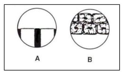
- The field of view in Image A (above) is 2 mm or 2000 µm.
- There are three cells that fit across the 2 mm/2,000-µm field (Image B).
- 2,000 ÷ 3 cells = 666 µm.
- Each cell is ~660 µm.
Viewing Specimens/Prepared Slides:
In the circles provided in this chapter, you will make sketches of each specimen/slide.

Genus and Species Name: __________________________________
Objective Lens Used: ___________________________
Estimated Size of Specimen: _____________________________