10.2: Modelling Predator-Prey Interactions

This material in this chapter has been adapted from Donovan and Welden (2002). 

Donovan, T. M. and C. Welden. 2002. Spreadsheet exercises in ecology and evolution. Sinauer Associates, Inc. Sunderland, MA, USA.

 

 

PREDATOR-PREY DYNAMICS

Objectives

• Develop a model for the interactions between predators and their prey.

• Understand how variation in prey demographic rates, predator demographic rates, and predator attack rates influence the population growth of predators and their prey.

 

INTRODUCTION

In this chapter, we will explore the classic Lotka-Volterra predator-prey model (Rosenzweig and MacArthur 1963), which treats each population as if it were growing exponentially.

 

 

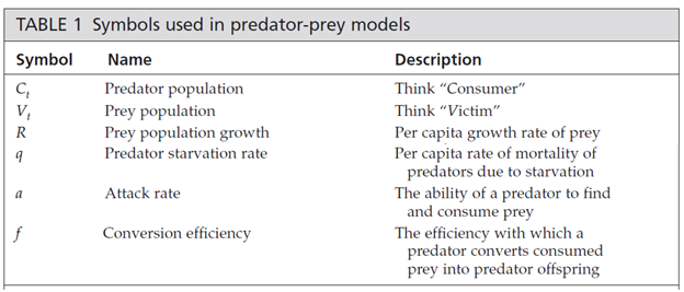
The Classical Lotka-Volterra Predator-Prey Model

In the classic Lotka-Volterra model, neither prey population nor predator population has an explicit carrying capacity. However, either or both may have an implicit carrying capacity imposed by the interaction between the two populations.

 

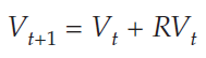
To model the prey population, we begin with a basic geometric model for the prey population

and subtract the number of prey individuals killed by predators in the interval from t  to t + 1. This number killed will depend on the number of predators: the more predators, the more prey they will kill. It will also depend on the number of prey available: the more prey, the more successful the predators. Finally, it will depend on the attack rate: the ability of a predator to find and consume prey. The number of prey killed in one time interval will be the product of these, or using the symbols given above, aC_tV_t. The equation for the prey population thus becomes

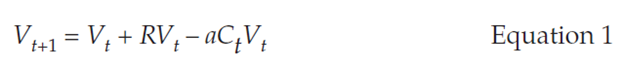
In words, the prey population grows according to its per capita growth rate minus losses to predators. Losses are determined by attack rate, predator population, and prey population.

 

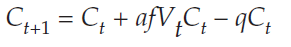
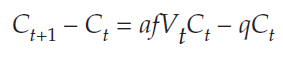
To model the predator population, we also begin with an exponential model, in concept. However, there is a wrinkle in this model, because we cannot assume a constant per capita rate of population growth. There is no simple R for the predator population because its growth rate will depend on how many prey are caught. As in the prey model, the number of prey caught will be aC_tV_t. The growth of the predator population will depend on this number, and on the efficiency with which predators convert consumed prey into predator offspring. We will represent this conversion efficiency with the parameter f, so the per capita population growth of predators will be afV_tC_t. We should reduce this predator population growth by some quantity to represent the starvation rate of predators who fail to consume prey. This will be the product of the per capita starvation rate times the predator population: qC_t. Taking all this into account, we can write an equation for the predator population:

In words, the predator population grows according to the attack rate, conversion efficiency, and prey population, minus losses to starvation. Note that the product afV_t acts as the predator’s R.

 

Having created these models, we can ask several questions about the interaction they portray, such as

• Under what conditions (i.e., parameter values) will the predator population drive the prey to extinction?

• Under what conditions will the predator population die off, leaving the prey population to expand unhindered?

• Under what conditions will predator and prey populations both persist indefinitely? What will be their population dynamics while they coexist? In other words, will one or both populations stabilize, or will they continue to change over time?

 

Equilibrium Solutions

As we did for the Interspecific Competition model, we will begin to answer these questions by seeking equilibrium solutions to Equations 1 and 2. For the prey population, we want to find values of predator and prey population sizes at which the prey population remains stable. In other words, we want to solve for ΔV_t = 0.

Beginning with Equation 1

we subtractV_t from both sides, and get

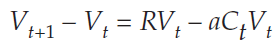
Because V_t+1 – V_t = ΔV_t we can substitute into the equation and get

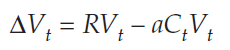
We are looking for a solution when ΔV_t = 0, so we substitute again:

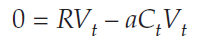
Adding aC_tV_t to both sides gives us

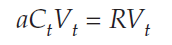
Dividing both sides byV_t, we get

Dividing both sides by a gives us our solution:

In words, the prey population reaches equilibrium when the predator population equals the prey’s per capita growth rate divided by the predator’s attack rate. Note that this is a constant. Strangely, the equilibrium size of the prey population is not determined by this solution, which says, in effect, that the prey population can be stable at any size as long as the predator population is at the specified size. 

 

For the predator population, we follow the same strategy, and solve for ΔC = 0. Beginning with Equation 2,

we subtract C_t  from both sides, and get

Because C_t+1 – C_t = ΔC_t, we can substitute into the equation and get

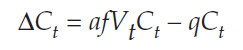
We are looking for a solution when ΔC_t = 0, so we substitute again:

Adding qC_t to both sides gives us

Dividing both sides by C_t, we get

 

 

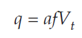
Dividing both sides by af gives us our solution:

In words, the predator population reaches equilibrium when the prey population equals the predator’s starvation rate over the product of attack rate times conversion efficiency.  Note that this is also a constant, and like the solution for the prey population, it does not specify the equilibrium size of the predator population, only the size of the prey population at which the predators are at equilibrium. 

 

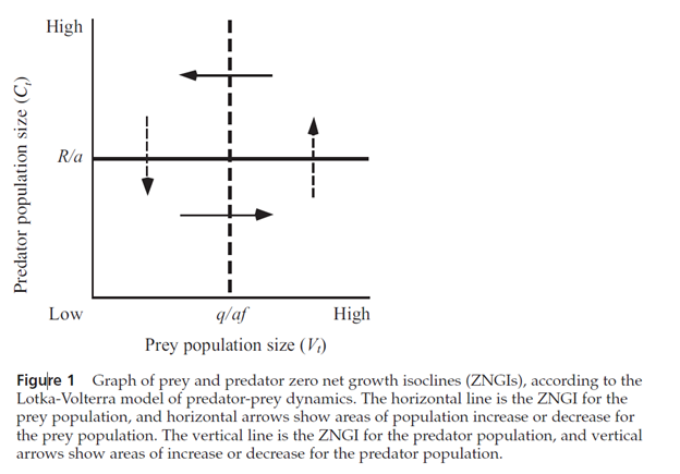
As we did in the model of interspecific competition, we can plot the population sizes of the two interacting populations on the two axes of a graph (Figure 1). The equilibrium solutions (Equations 3 and 4) then become straight-line zero net growth isoclines (ZNGIs), as they did in the interspecific competition model.

On this graph, the ZNGI for the prey population is a horizontal line at Ct = R/a (the solid line in Figure 1), below which the prey population increases, and above which it decreases (solid arrows).

The ZNGI for the predator population is a vertical line at V_t = q/af (dashed line), to the left of which the predator population decreases, and to the right of which it increases (dashed arrows).

Where the two lines cross, the two populations are at equilibrium. As in the Interspecific Competition exercise, the two populations are represented by a point on this phase diagram, and that point will trace out a trajectory through phase space as the populations change in size.

As discussed in most ecology texts, the continuous-time Lotka-Volterra model predicts that the point representing the two populations will cycle endlessly around the point where the two ZNGIs cross.

 

 

LITERATURE CITED

King, A. A. and W. M. Schaffer. 2001. The geometry of a population cycle: A mechanistic model of snowshoe hare demography. Ecology 82: 814–830.

Rosenzweig, M. L. and R. H. MacArthur. 1963. Graphical representation and stability conditions of predator-prey interactions. American Naturalist 97: 209–223.

 

 

ES 211 – Lokta-Volterra Terms Sheet

The terms we will use in ES 211 are slightly different than those above. The equations in the terms sheet below are the same as the equations shown above for ΔC (“consumer”, in our sheet, dN_pred/dt) and ΔV (“victim”, in our sheet dN_prey/dt)

 

 

dN_prey/dt = rate of change in prey population (change in number over change in time)

dN_pred/dt = rate of change in predator population (change in number over change in time)

c = rate at which prey are converted into offspring (a slope: predators produced per predator per time as a function of prey consumed per unit time)

p = attack rate efficiency (a slope: the change in prey consumed per predator per time as a function of the number of prey); higher search or handling time leads to a lower p

d_pred = predator death rate

r_prey = prey per capita rate of increase

N_prey = number of prey

N_pred = number of predators

Isocline of Zero Growth for Prey occurs at N_pred = r_prey/p 

Isocline of Zero Growth for Predator occurs at N_prey = d/cp