10.1: Modelling Competition

This material in this chapter has been adapted from Donovan and Welden (2002). 

Donovan, T. M. and C. Welden. 2002. Spreadsheet exercises in ecology and evolution. Sinauer Associates, Inc. Sunderland, MA, USA.

 

 

INTERSPECIFIC COMPETITION AND COMPETITIVE EXCLUSION

 

Objectives

• Understand the components of the Lotka-Volterra model of interspecific competition.

• Use the model to explore competitive exclusion and coexistence.

• Determine under what conditions two competing species can coexist, in terms of their competition coefficients, carrying capacities, and intrinsic rates of increase.

 

INTRODUCTION

Our previous discussions of population dynamics considered only one population. As informative as those models were, it should be obvious that real populations do not exist in isolation, but share habitats with populations of other species. In many cases, coexisting species will interact by interspecific competition, predation, parasitism, mutualism, or other ecological interactions. More realistic models must take such interactions into account. In the 1920s, Vito Volterra and Alfred Lotka (1932) independently developed models of interspecific competition (competition between two species), and investigated the conditions that would permit competing species to coexist indefinitely.

An important ecological generalization, the competitive exclusion principle, has grown out of the Lotka-Volterra model and from other sources. This principle states that two species cannot coexist unless their niches are sufficiently different that each limits its own population growth more than it limits that of the other. In other words, if there is too much niche overlap, one species will competitively exclude the other. In reality, whether two species coexist depends not only on their competitive interactions with each other, but also on their interactions with the abiotic environment and with other species not included in this simple model. Nevertheless, the competitive exclusion principle has proven fruitful in stimulating research and understanding ecological interactions in the natural world.

 

Model Development

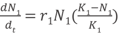
The logistic model of population growth focuses on intraspecific competition (competition between individuals of the same species). To keep things (relatively) simple, we will develop our model of interspecific competition beginning with this form of the logistic model:

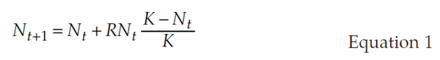
where K is the carrying capacity, or largest sustainable population. The value of K is set by available resources and by each individual’s resource demand. This version of the logistic model has intraspecific competition built into it in the term (K – N_t)/K. This term reduces the population growth rate in response to the addition of each new member of the population, representing the reduction in per capita birth rate, and increase in per capita death rate, caused by competition for limited resources.

The Lotka-Volterra model of interspecific competition builds on the logistic model of a single population. It begins with a separate logistic model of the population of each of the two competing species.

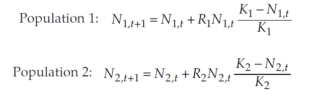
Note the use of subscripts 1 and 2 to denote which species’ population is being modeled. Each population has its own rate of increase R and carrying capacity K, and these may differ between the two species.

Next, we build interspecific competition into each of these equations. In the model of population 1 above, we assume that each new member of population 1 reduces resources available to each member of population 1, and thus reduces population growth rate. In two-species model, new members of population 2 will also reduce resources available to members of population 1—this is, after all, the meaning of interspecific competition.

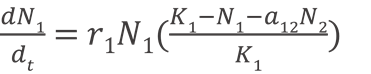
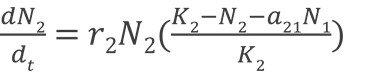
The simplest way to model this would be to modify the (K1 – N_1,t)/K term into (K₁ – N_1,t – N_2,t)/K₁. However, this assumes that each additional member of population 2 will affect population 1 exactly as much as an additional member of population 1. That is not necessarily the case, so we multiply N2,t in this term by a competition coefficient, a12 to express how much effect each additional member of population 2 has on population 1, relative to the effect of a new member of population 1. We modify the model for population 2 in a parallel way. The resulting Lotka-Volterra model of two-species competition is:

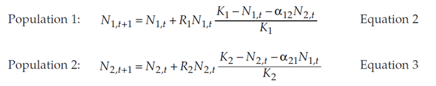
Note the subscripts on the competition coefficients: a₁₂ expresses the effect of one member of population 2 on the growth rate of population 1; a₂₁ expresses the effect of one member of population 1 on the growth rate of population 2.

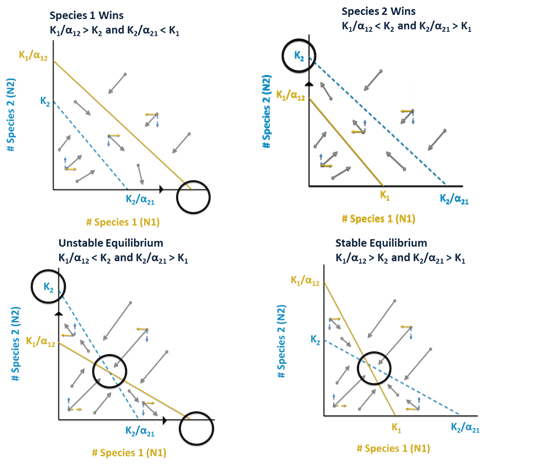
In broad terms, the question Lotka and Volterra asked was, What will happen to the population dynamics of these two populations, given various values of the model parameters? Are there parameter values that will produce a winner and a loser—one population that persists while the other goes extinct? This would be competitive exclusion. Will other values result in coexistence, in which both competing populations persist indefinitely?

 

Equilibrium Solutions

One approach to answering the questions posed above is to look for equilibrium solutions to Equations 2 and 3. In words, the population stops growing when it is at equilibrium, which should come as no surprise. This equation is satisfied if N_1,t = 0 or if R₁ = 0, but these solutions are trivial.

The equation is also satisfied by the more interesting case of

If we add N_1,t to both sides and rearrange the terms, we get

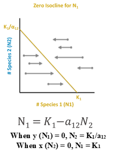
Notice that this equation is in the general form of a linear equation, y = a + bx, and is therefore a straight line. We call this line a zero net growth isocline, or ZNGI, because anywhere along it, population 1 has zero net growth. In other words, this is an equilibrium solution for population 1.

Just as x and y in the general linear equation y = a + bx can be used as coordinates for graphing, so we can use N1,t and N2,t as coordinates to graph Equation 4. We can graph this isocline by finding any two points along it and connecting them with a straight line. Two convenient points are where N2,t = 0 and where N1,t = 0. 

If N_2,t = 0, then we solve for N_1,t. Equation 4 becomes

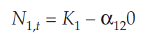
Which reduces to

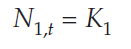
In words, if there are no members of population 2 in the habitat, population 1 will stabilize at its own carrying capacity, K₁. This seems a reasonable solution.

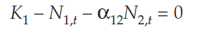
If we set N_1,t = 0, and then solve for N_2,t. Equation 4 becomes

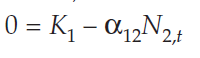
and adding a₁₂N_2,t to both sides gives us

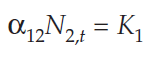
Dividing both sides by a₁₂ gives us

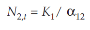
In words, if there are K₁/a₁₂ members of population 2 in the habitat, there will be no resources left over for population 1, and its numbers will go to zero.

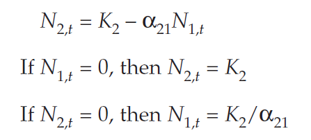
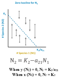
We can find a ZNGI and two points on it for population 2 in the same manner.

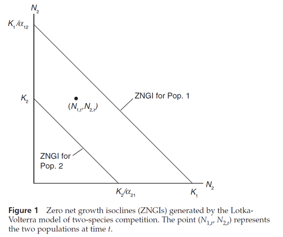
We can draw these isoclines on a linear graph of the two populations as shown in Figure 1. If we plot N₁ on the horizontal axis and N₂ on the vertical, then the solution points found become the intercepts of the isoclines on the axes.

We can graph the populations of the two species at any time by a point on a graph. If the point falls below and/or to the left of a species’ isocline, that population will continue to increase. If the point falls above and/or to the right of a species’ isocline, that population will decrease. In the case of the point shown in Figure 1, population 1 will increase and population 2 will decrease. As time passes, the point will move downward (population 2 decreases) and to the right (population 1 increases), and the point describing the two populations will trace some trajectory across the graph.

Notice that time does not appear on either axis of this graph. Figure 1 is called a phase diagram, and the space bounded by its axes is called phase space. You can plot the trajectory of two changing populations through the phase space and from that determine whether one species excludes the other, or if they coexist. The isoclines need not be arranged as shown in Figure 1; their arrangement will depend on the values of K₁, K₂, a₁₂, and a₂₁.

 

LITERATURE CITED

Lotka, A. J. 1932. The growth of mixed populations: two species competing for a common food supply. Journal of the Washington Academy of Sciences 22: 461–469.

 

 

 

 

 

 

Summary of Models to Know  – Exponential, Logistic, Competition 

 

Exponential (Review) – No Carrying Capacity

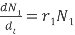
r₁ = intrinsic growth rate of species 1

N₁ = population size of species 1

 

Logistic (Review) – Single Species, Carry Capacity

K₁ = carrying capacity of species 1 (when K = N, dN/dt = 0)

 

Competition – Two Species Logistic Model, Equations Linked

α₁₂ or α = a measure of the per capita effect of species 2 on the growth of species 1

α₂₁ or β = a measure of the per capita effect of species 1 on the growth of species 2

 

 

Species 1 and Species 2 Isoclines

 

 

 

 

 

 

 

 

 

 

 

 

 

Species 1 and Species 2 Outcomes