7.3: Leslie Matrix Models

This material in this chapter has been adapted from Donovan and Welden (2002) and from Wikipedia (Leslie matrix entry). 

Donovan, T. M. and C. Welden. 2002. Spreadsheet exercises in ecology and evolution. Sinauer Associates, Inc. Sunderland, MA, USA.

 

Age-Structured Leslie Matrix Models

 

OBJECTIVES

• Set up a model of population growth with age structure.

• Estimate the finite rate of increase from Leslie matrix calculations.

 

INTRODUCTION: AGE-STRUCTURED MODELS

You’ve probably seen the geometric growth formula many times by now. It has the form

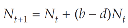
where b is the per capita birth rate and d is the per capita death rate for a population that is growing in discrete time. The term (b-d)N_t is the same as the term (B-D). Here, b and d refer to rates that need to be multiplied by N_t (the population size at time t) to find the absolute number of births (B) and deaths (D). Note that the equation above ignores immigration (I) and emigration (E), and it therefore assumes that we are working with a closed population.

The term (b – d) is so important in population biology that it is given its own symbol, R. It is called the intrinsic (or geometric) rate of natural increase, and represents the per capita rate of change in the size of the population. Substituting R for b – d gives

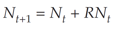
We can factor N_t out of the terms on the right-hand side, to get

 

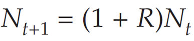
The quantity (λ + R) is called the finite rate of increase, λ. Thus, we can write

where N is the number of individuals present in the population, and t is a time interval of interest. This equation says that the size of a population at time t + 1 is equal to the size of the population at time t multiplied by a constant, λ. When λ = 1, the population will remain constant in size over time. When λ < 1, the population declines geometrically, and when λ > 1, the population increases geometrically. Although geometric growth models have been used to describe population growth, like all models they come with a set of assumptions. 

What are the assumptions of the geometric growth model? The equations describe a population in which there is no genetic structure, no age structure, and no sex structure to the population (Gotelli 2001), and all individuals are reproductively active when the population census is taken. The model also assumes that resources are virtually unlimited and that growth is unaffected by the size of the population. Can you think of an organism whose life history meets these assumptions? Many natural populations violate at least one of these assumptions because the populations have structure: They are composed of individuals whose birth and death rates differ depending on age, sex, or genetic makeup. All else being equal, a population of 100 individuals that is composed of 35 pre-reproductive age individuals, 10 reproductive-age individuals, and 55 post-reproductive age individuals will have a different growth rate than a population where all 100 individuals are of reproductive age. In this section, you will learn how to use the matrix model to explore the growth of populations that have age structure and estimate λ for structured populations.

 

Leslie Matrix Model Notation

In applied mathematics, the Leslie matrix is a discrete, age-structured model of population growth that is very popular in population ecology. The Leslie matrix (also called the Leslie model) is one of the most well-known ways to describe the growth of populations (and their projected age distribution), in which a population is closed to migration, growing in an unlimited environment, and where only one sex, usually the female, is considered.

The Leslie matrix is used in ecology to model the changes in a population of organisms over a period of time. In a Leslie model, the population is divided into groups based on age classes. At each time step, the population is represented by a vector with an element for each age class where each element indicates the number of individuals currently in that class.

Let us begin with some notation often used when modeling populations that are structured (Caswell 2001; Gotelli 2001). For modeling purposes, we divide individuals into groups by either their age or their age class. Although age is a continuous variable when individuals are born throughout the year, by convention individuals are grouped or categorized into discrete time intervals. That is, the age class of 3-year-olds consists of individuals that just had their third birthday, plus individuals that are 3.5 years old, 3.8 years old, and so on. In age-structured models, all individuals within a particular age group (e.g., 3-year-olds) are assumed to be equal with respect to their birth and death rates. The age of individuals is given by the letter x, followed by a number within parentheses. Thus, newborns are x(0) and 3-year-olds are x(3). In contrast, the age class of an individual is given by the letter i, followed by a subscript number. A newborn enters the first age class upon birth (i1), and enters the second age class upon its first birthday (i2). Caswell (2001) illustrates the relationship between age and age class as:

 

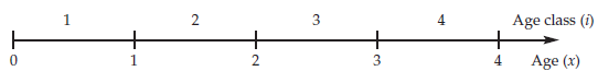
Thus, whether we are dealing with age classes or ages, individuals are grouped into discrete classes that are of equal duration for modeling purposes. A typical life cycle of a population with age-class structure is:

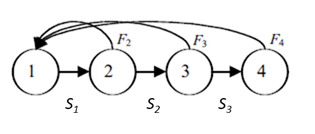
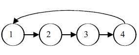
The age classes or ages are represented by circles. In this example, we are considering a population with just four ages. The horizontal arrows between the circles represent survival probabilities, Sx—the probability that an individual of age x will survive to age x + 1. Note that age four has no arrow leading to age five, indicating that the probability of surviving to the age five class is 0. The curved arrows at the top of the diagram represent births. These arrows all lead to age 1 because newborns, by definition, enter the first age upon birth. Because “birth” arrows emerge from ages 2, 3, and 4 in the above example, the diagram indicates that individuals that are all three of these ages can reproduce. Note that individuals that are only age 1 do not reproduce. If only individuals of age class 4 reproduced, our diagram would have to be modified:

 

Calculating Lambda using the Leslie Matrix Model

The major goal of the matrix model is to compute λ, the finite rate of increase in Equation 1, for a population with age structure. In our matrix model, we can compute the time-specific growth rate as λ_t. The value of λ_t can be computed as:

This time-specific growth rate is not necessarily the same λ in Equation 1. To determine Nt and Nt+1, we need to count individuals at some standardized time period over time. We will make two assumptions in our computations. First, we will assume that the time step between Nt and Nt+1 is one year, and that age classes are defined by yearly intervals. This should be easy to grasp, since humans typically measure time in years and celebrate birthdays annually. Second, we will assume for this exercise that our population censuses are completed once a year, immediately after individuals breed (a post-breeding census). The number of individuals in the population in a census at time t + 1 will depend on how many individuals of each age class were in the population at time t, as well as the birth and survival probabilities for each age class. Let us start by examining the survival probability, S_x, which you may remember from life tables. S_x represents the number of individuals surviving from age class x to age class x + 1

If we consider survival alone, we can compute the number of individuals of age class 2 at time t + 1 as the number of individuals of age class 1 at time t multiplied by S1.

This equation works for calculating the number of individuals at time t + 1 for each age class in the population except for the first, because individuals in the first age class arise only through birth. Now let’s consider birth rates. There are many ways to describe the occurrence of births in a population. Here, we will assume a simple birth-pulse model, in which individuals give birth the moment they enter a new age class. When populations are structured, the birth rate is called the fecundity, or the average number of offspring born per unit time to an individual female of a particular age. Individuals that are of pre-reproductive or post-reproductive age have fecundities of 0. Individuals of reproductive age typically have fecundities > 0. Here, we will write fecundity as m_x, the average female offspring per female of a given age in the population

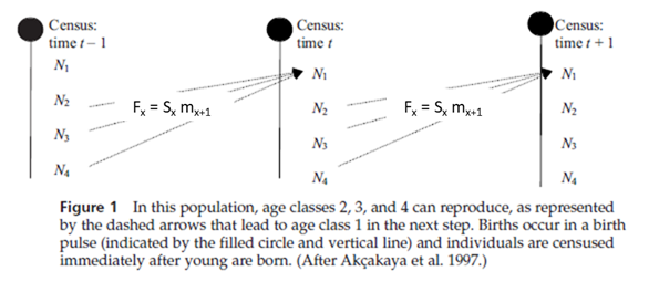
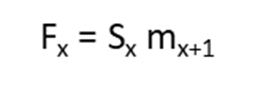
Figure 1 is a hypothetical diagram of a population with four age classes that are censused at three time periods: time t – 1, time t, and time t + 1. In Figure 1, all individuals “graduate” to the next age class on their birthday, and since all individuals have roughly the same birthday, all individuals counted in the census are “fresh”; that is, the newborns were just born, individuals in age class 2 just entered age class 2, and so forth. Figure 1 shows that the number of individuals in the first age class at time t depends on the number of breeding adults in the previous time step. If we knew how many adults actually bred in the previous time step, we could compute fecundity, or the average number of offspring born per unit time per individual (Gotelli: 2001). However, the number of adults is not simply N2 and N3 and N4 counted in the previous time step’s census; these individuals must survive a long period of time (almost a full year until the birth pulse) before they have another opportunity to breed. Thus, we need to discount the fecundity, m_x, by the probability that an adult will actually survive from the time of the census to the birth pulse (S_x), (Gotelli 2001). These adjusted estimates, which are used in matrix models, are called fertilities and are designated by the letter F.

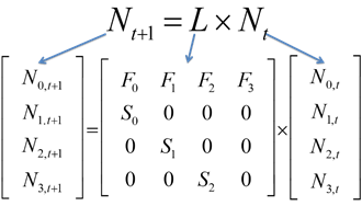
Leslie (1945) developed a matrix method for predicting the size and structure of next year’s population for populations with age structure. The Leslie Matrix is a square matrix with the same number of rows and columns as the population vector has elements. The (i,j)th cell in the matrix indicates how many individuals will be in the age class i at the next time step for each individual in stage j. At each time step, the population vector (N_t) is multiplied by the Leslie matrix (L) to generate the population vector for the subsequent time step (N_t+1).

 

Since our population has only four ages, the Leslie matrix is a four row by four column matrix. If our population had five ages, the Leslie matrix would be a five row by five column matrix. The fertility rates of ages 1 through 4 are given in the top row. Most matrix models consider only the female segment of the population, and define fertilities in terms of female offspring. The survival probabilities, Sx, are given in the sub-diagonal; S1 through S3 are survival probabilities from one age to the next. For example, S1 is the probability of individuals surviving from age 1 to age 2. All other entries in the Leslie matrix are 0. The composition of our population can be expressed as a column vector, N_t, which is a matrix that consists of a single column. Our column vector will consist of the number of individuals in age classes 1, 2, 3, and 4.

When the Leslie matrix, L, is multiplied by the population vector, N_t, the result is another population vector (which also consists of one column); this vector is called the resultant vector N_t+1 and provides information on how many individuals are in age classes 1, 2, 3, and 4 in year t + 1.

 

 

The multiplication works as follows:

 

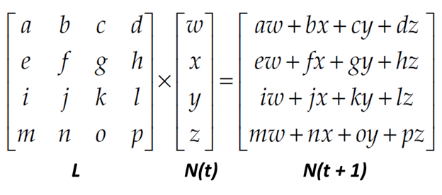
The first entry in the resultant vector is obtained by multiplying each element in the first row of the L matrix by the corresponding element in the N_t vector, and then summing the products together. In other words, the first entry in the resultant vector N_t+1 equals the total of several operations: multiply the first entry in the first row of the L matrix by the first entry in N_t vector, multiply the second entry in the first row of the L matrix by the second entry in the N_t vector, and so on until you reach the end of the first row of the L matrix, then add all the products.

 

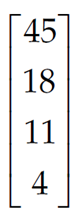
For example, assume that you have been following a population that consists of 45 individuals in age class 1, 18 individuals in age class 2, 11 individuals in age class 3, and 4 individuals in age class 4. The initial vector of abundances is written

 

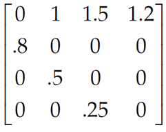
Assume that the Leslie matrix for this population is

Following Equation 4, the number of individuals of age classes 1, 2, 3, and 4 at time t + 1 would be computed as

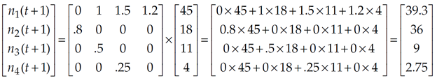
The time-specific growth rate, λ_t, can be computed as the total population at time t +1 divided by the total population at time t. For the above example,

 

As we mentioned earlier, λ_t is not necessarily equal to λ in Equation 1. The Leslie matrix not only allows you to calculate λ_t (by summing the total number of individuals in the population at time t + 1 and dividing this number by the total individuals in the population at time t), but also to evaluate how the composition of the population changes over time. If you multiply the Leslie matrix by the new vector of abundances, you will project population size for yet another year. Continued multiplication of a vector of abundance by the Leslie matrix eventually produces a population with a stable age distribution, where the proportion of individuals in each age class remains constant over time, and a stable (unchanging) time-specific growth rate, λ_t. When the λ_t’s converge to a constant value, this constant is an estimate of l in Equation 1. Note that this l has no subscript associated with it. Technically, l is called the asymptotic growth rate when the population converges to a stable age distribution. At this point, if the population is growing or declining, all age classes grow or decline at the same rate.

 

LITERATURE CITED

Akçakaya, H. R., M. A. Burgman, and L. R. Ginzburg. 1997. Applied Population Ecology. Applied Biomathematics, Setauket, NY.

Caswell, H. 2001. Matrix Population models, Second Edition. Sinauer Associates, Inc. Sunderland, MA.

Gotelli, N. 2001. A Primer of Ecology, Third Edition. Sinauer Associates, Sunderland, MA.

Leslie, P. H. 1945. On the use of matrices in certain population mathematics. Biometrika 33: 183–212.