7.2: Life Tables

This material in this chapter has been adapted from Donovan and Welden (2002).

Donovan, T. M. and C. Welden. 2002. Spreadsheet exercises in ecology and evolution. Sinauer Associates, Inc. Sunderland, MA, USA.

 

Objectives

·         Use age or stage-specific abundance data to calculate a variety of life table parameters.

·         Discover how patterns of survivorship relate to the classic three types of survivorship curves.

·         Learn how patterns of survivorship relate to life expectancy.

·         Explore how patterns of survivorship and fecundity affect rate of population growth.

 

INTRODUCTION

A life table is a record of survival and reproductive rates in a population, broken out by age, size, or developmental stage (e.g., egg, hatchling, juvenile, adult). Ecologists and demographers (scientists who study human population dynamics) have found life tables useful in understanding patterns and causes of mortality, predicting the future growth or decline of populations, and managing populations of endangered species.

Predicting the growth and decline of human populations is one very important application of life tables. As you might expect, whether the population of a country or region increases or decreases depends in part on how many children each person has and the age at which people die. But it may surprise you to learn that population growth or decline also depends on the age at which they have their children.

Another use of life tables is in species conservation efforts, such as in the case of the loggerhead sea turtle of the southeastern United States (Crouse et al., 1987). Generally speaking, the loggerhead population is declining and mortality among loggerhead eggs and hatchlings is very high. These facts led conservation biologists to advocate for the protection of nesting beaches. When these measures proved ineffective in halting the population decline, compiling and analyzing a life table for loggerheads indicated that reducing mortality of older turtles would have a greater probability of reversing the population decline. Therefore, management efforts shifted to persuading fishermen to install turtle exclusion devices on their nets to prevent older turtles from drowning.

 

Life Table Varieties

Life tables come in two varieties: cohort and static. A cohort life table follows the survival and reproduction of all members of a cohort from birth to death. A cohort is the set of all individuals born, hatched, or recruited into a population during a defined time interval. Cohorts are frequently defined on an annual basis (e.g., all individuals born in 1978), but other time intervals can be used as well.

A static life table records the number of living individuals of each age in a population and their reproductive output. The two varieties have distinct advantages and disadvantages, some of which we discuss below.

Life tables (whether cohort or static) that classify individuals by age are called age-based life tables. Such life tables treat age the same way we normally do: that is, individuals that have lived less than one full year are assigned age zero; those that have lived one year or more but less than two years are assigned age one; and so on. Life tables represent age by the letter x, and use x as a subscript to refer to survivorship, fecundity, and so on, for each age.

 

Size-based and stage-based life tables classify individuals by size or developmental stage, rather than by age. Size-based and stage-based tables are often more useful or more practical for studying organisms that are difficult to classify by age, or whose ecological roles depend more on size or stage than on age.

 

• Cohort Life Tables

To build a cohort life table for, let’s say, humans born in the United States during the year 1900, we would record how many individuals were born during the year 1900, and how many survived to the beginning of 1901, 1902, etc., until there were no more survivors. This record is called the survivorship schedule.

We must also record the fecundity schedule—the number of offspring born to individuals of each age. The total number of offpsring is usually divided by the number of individuals in the age, giving the average number of offspring per individual, or per capita fecundity.

Many life tables count only females and their female offspring; for animals with two sexes and equal numbers of males and females of each age, the resulting numbers are the same as if males and females were both counted. For most plants, hermaphroditic animals, and many other organisms, distinctions between the sexes are nonexistent or more complex, and life table calculations may have to be adjusted.

 

• Static Life Tables

A static life table is similar to a cohort life table but introduces a few complications. For many organisms, especially mobile animals with long life spans, it can be difficult or impossible to follow all the members of a cohort throughout their lives. In such cases, population biologists often count how many individuals of each age are alive at a given time. That is, they count how many members of the population are currently in the 0–1- year-old class, the 1–2-year-old class, etc.

These counts can be used as if they were counts of survivors in a cohort, and all the calculations described below for a cohort life table can be performed using them. In doing this, however, the researcher must bear in mind that she or he is assuming that age-specific survivorship and fertility rates have remained constant since the oldest members of the population were born. This is usually not the case and can lead to some strange results, such as negative mortality rates. These are often resolved by averaging across several ages, or by making additional assumptions.

 

 

Life Table Parameters

 Survivorship and fecundity schedules are the raw data of any life table. From them we can calculate a variety of other quantities, including age-specific rates of survival, mortality, fecundity, survivorship curves, life expectancy, generation time, net reproductive rate, and intrinsic rate of increase. Which of these quantities you calculate will depend on your goals in constructing the life table.

 

Key Parameters

x and n_x When conducting a study, these are the data generally collected on populations. We then calculate the rest of the life table from these data.

• x The first column, represents the age classes. This column could represent days, minutes, or life stages (eggs, juveniles, adults, etc.).
• n_x The number of individuals from the original cohort that are alive at the specified age, age class, or life stage (x).

 

From information on the number of individuals at each age, we can calculate a variety of survival and mortality rates.

• d_x The difference between the number of individuals alive for any age class (n_x) and the next older age class (n_x+1) is the number of individuals that have died during that time intervals. d_x is a measure of age-specific mortality.
• q_x The number of individuals that died during any given time interval (d_x) divided by the number alive at the beginning of that interval (n_x) provides an age-specific mortality rate.
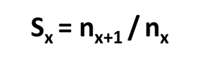
• S_x The age-specific survival rate for age interval x is the proportion of individuals that survive during any given time interval.
• l_x The number of individuals surviving to any given life stage as a proportion of the original cohort size. l_x represents the probability at birth of surviving to any given life stage.

 

Calculating life expectancy (E_x) requires calculating two additional parameters, L_x and T_x.

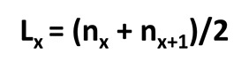
• L_x  The number of individuals that are alive in the middle of the first age class – 0.5 years old, or 1.5 years old.
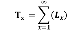
• T_x The total years lived into the future by individuals in age class x. This value is calculated by summing the values of Lx cumulatively from age x to the end of the life table. The number of time units left for all individuals to live from age x onward – obtained by summing the L_xs.
• E_x The life expectancy for an individual of age x is age-specific life expectancy divided by number of individuals at age x. Life expectancy represents the average additional length of times than an individual will live once it has reached age x.

 

A typical life table is shown in Figure 1. If we were to build a cohort life table for a population born during the year 1900, we would record how many individuals were born during the year 1900, and how many survived to the beginning of 1901, 1902, etc., until there were no more survivors. This record is called the survivorship schedule. We would also record the fecundity schedule: the number of offspring born to members of each age class. The total number of offspring is usually divided by the number of individuals in the age class, giving the average number of offspring per individual, which is represented by bx.

 

Figure 1: A cohort of 3751 individuals tracked over time. The number alive at the beginning of each year is given in Column B, and the average number of offspring per female is given in Column C. Columns D through G are calculated from information in columns A through C.

 

 

Mt. Olivet Cemetary was taken by Daniel Lobo and is licensed under Creative Commons Attribution 2.0 Generic.

 

Calculating Key Parameters

Standardized Survival Schedule (l_x). Because we want to compare cohorts of different initial sizes, we standardize all cohorts to their initial size at time zero, n₀. We do this by dividing each nx by n₀. This proportion of original numbers surviving to the beginning of each interval is denoted lx, and calculated as

We can also think of lx as the probability that an individual survives from birth to the beginning of age x. Because we begin with all the individuals born during the year (or other interval), lx always begins at a value of one (i.e., n₀/n₀), and can only decrease with time. At the last age, k, n_k is zero.

 

Age-Specific Survivorship (Sx). Standardized survivorship, l_x, gives us the probability of an individual surviving from birth to the beginning of age x. But what if we want to know the probability that an individual who has already survived to age x will survive to age x + 1? We calculate this age-specific survivorship as S_x = l_x+1/l_x, or equivalently,

 

Life Expectancy (E_x). You may have heard another demographic statistic, life expectancy, mentioned in discussions of human populations. Life expectancy is how much longer an individual of a given age can be expected to live beyond its present age. Life expectancy is calculated in three steps.

First, we compute the proportion of survivors at the mid-point of each time interval (L_x—note the capital L here); that is,

Second, we sum all the L_x values from the age of interest (n) up to the oldest age, k:

Finally, we calculate life expectancy as

Life expectancy is age-specific—it is the expected number of time-intervals remaining to members of a given age. The statistic most often quoted (usually without qualification) is the life expectancy at birth (E₀).

 

Survivorship Curves

There are three classic survivorship curves, called Type I, Type II, and Type III (Figure 2). To understand survivorship curves you can use survivorship schedules (Sx) to calculate and graph standardized survivorship (l_x), age-specific survivorship (g_x), and life expectancy (e_x).

 

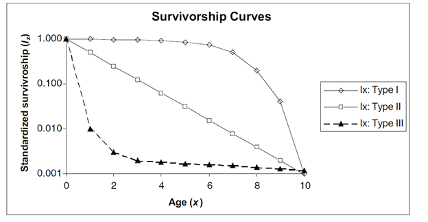
Figure 2: Hypothetical survivorship curves. Note that the y-axis has a logarithmic scale. Type 1 organisms have high survivorship throughout life until old age sets in, and then survivorship declines dramatically to 0. Humans are type 1 organisms. Type III organisms, in contrast, have very low survivorship early in life, and few individuals live to old age.

 

 

Population Growth or Decline

We frequently want to know whether a population can be expected to grow, shrink, or remain stable, given its current age-specific rates of survival and fecundity. We can determine this by computing the net reproductive rate (R₀). To predict long-term changes in population size, we must use this net reproductive rate to estimate the intrinsic rate of increase (r).

 

Net Reproductive Rate (R₀) We calculate net reproductive rate (R₀) by multiplying the standardized survivorship of each age (l_x) by its fecundity (b_x), and summing these products:

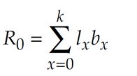
The net reproductive rate is the lifetime reproductive potential of the average female, adjusted for survival. Assuming survival and fertility schedules remain constant over time, if R₀ > 1, then the population will grow exponentially. If R₀ < 1, the population will shrink exponentially, and if R₀ = 1, the population size will not change over time. You may be tempted to conclude the R₀ = r, the intrinsic rate of increase of the exponential model. However, this is not quite correct, because r measures population change in absolute units of time (e.g., years) whereas R₀ measures population change in terms of generation time. To convert R₀ into r, we must first calculate generation time (G), and then adjust R₀.

 

Generation Time. Generation time is calculated as

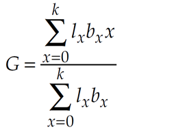
For organisms that live only one year, the numerator and denominator will be equal, and generation time will equal to one year. For all longer-lived organisms, generation time will be greater than one year, but exactly how much greater will depend on the survival and fertility schedules. Along-lived species that reproduces at an early age may have a shorter generation time than a shorter-lived one that delays reproduction.

 

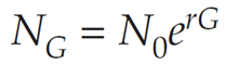
Intrinsic Rate of Increase. We can use our knowledge of exponential population growth and our value of R₀ to estimate the intrinsic rate of increase (r) (Gotelli 2001). The size of an exponentially growing population at some arbitrary time t is N_t = N₀ert, where e is the base of the natural logarithms and r is the intrinsic rate of increase. If we consider the growth of such a population from time zero through one generation time, G, it is

Dividing both sides by N₀ gives us

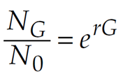
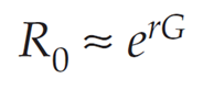
We can think of N_G /N₀ as roughly equivalent to R₀; both are estimates of the rate of population growth over the period of one generation.

 

Substituting R₀ into the equation gives us

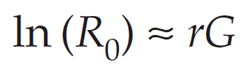
Taking the natural logarithm of both sides gives us

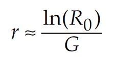
and dividing through by G gives us an estimate of r:

Finally, we can use our estimate of r (uncorrected or corrected) to predict the size of the population in the future. This kind of analysis is done for human populations to predict the effects of changes in medical care and birth control programs. If we assume that all age groups are roughly equivalent in size, a similar analysis can be done for endangered species to determine what intervention may be most effective in promoting population growth. The same analysis can be applied to pest species to determine what intervention may be most effective in reducing population size.

 

Reproductive Value

The idea that different individuals have different “value” in terms of their contribution to future generations is called their reproductive value (Fisher 1930). As Caswell (2001) states, “The amount of future reproduction, the probability of surviving to realize it, and the time required for the offspring to be produced all enter into the reproductive value of an age-class.”

The reproductive value of an individual of age x is designated at Vx, and is the number of offspring that an individual is expected to produce over its remaining life span (after adjusting for the growth rate of the population). Biologists are often interested in knowing the “value” of the different individuals from a practical standpoint because knowing something about the reproductive value can suggest which individuals should be harvested, killed, transplanted, etc. from a conservation or management perspective.

The reproductive value of different ages is strongly tied to an organism’s life history. Typically, reproductive value is low at birth, increases to a peak near the age of first reproduction, and then declines (Caswell 2001).

 

 

LITERATURE CITED

Caswell, H. 2001. Matrix Population Models, 2nd Ed. Sinauer Associates, Sunderland, MA.

Connell, J. H. 1970. A predator-prey system in the marine intertidal region. I. Balanus glandula. Ecological Monographs 40: 49–78. (Reprinted in Ecology: Individuals, Populations and Communities, 2nd edition, M. Begon, J. L. Harper and C. R. Townsend.. (1990) Blackwell Scientific Publications, Oxford.) 

Crouse, D. T., L. B. Crowder, and H. Caswell. 1987. A stage-based population model for loggerhead sea turtles and implications for conservation. Ecology 68: 1412–1423. 

Deevey, E. S., Jr. 1947. Life tables for natural populations of animals. The Quarterly Review of Biology 22: 283–314. (Reprinted in Readings in Population and Community Ecology, W.E. Hazen (ed.). 1970, W.B. Saunders, Philadelphia.) 

Fisher, R. A. 1930. The Genetical Theory of Natural Selection. Clarendon Press, Oxford.

Gotelli, Nicholas J. 2001. A Primer of Ecology, 3rd Edition. Sinauer Associates, Sunderland, MA.