
16.2: Quantifying Predator-Prey Dynamics
- Page ID
- 83706
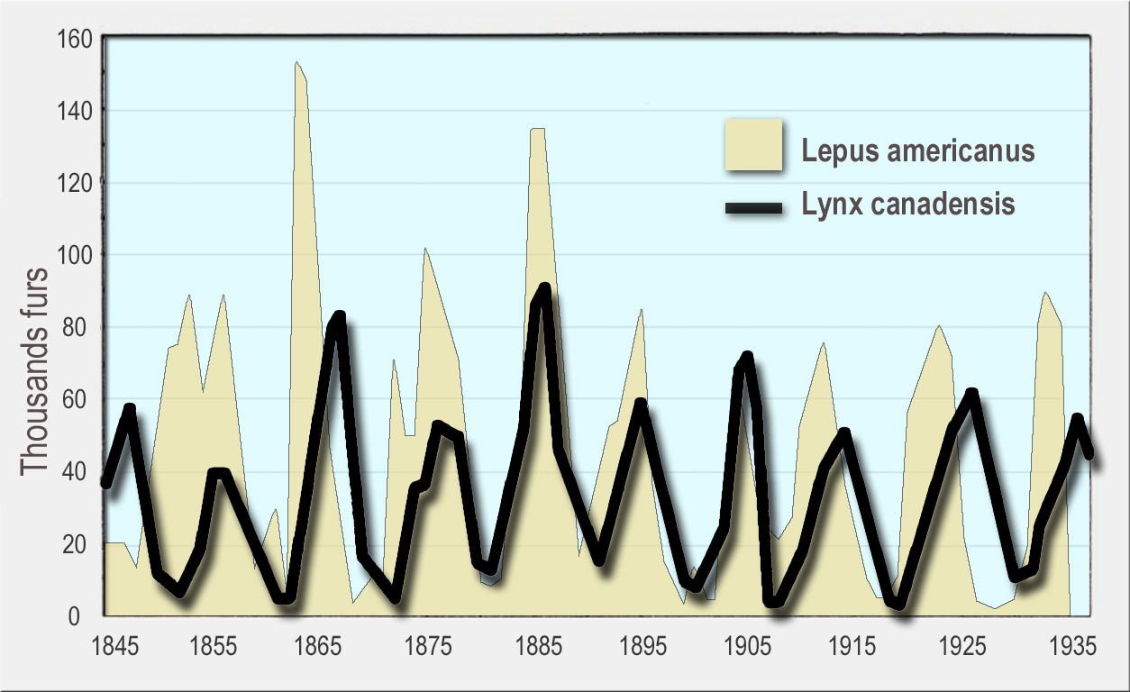
Figure \(\PageIndex{1}\): Numbers of snowshoe hare (Lepus americanus) (yellow background) and Canada lynx (black line, foreground) furs sold to the Hudson's Bay Company from 1845 to 1935. Image by Lamiot is licensed under CC BY-SA 4.0.
In the classic Lotka-Volterra model of predator-prey dynamics, both predators and prey are modeled using a modified version of the equation for exponential growth, so neither population has an explicit carrying capacity. However, either or both may have an implicit carrying capacity imposed by the interaction between the two populations.
To model the prey population, we begin with a basic exponential model with some additional terms. Here, the prey population is growing at their intrinsic growth rate rprey, but is also declining due to predation.
The number of prey killed will depend on the number of predators: the greater the number of predators, the more prey they will kill (Npred). It will also depend on the number of prey available: the more prey, the more successful the predators (Nprey). Finally, it will depend on the attack rate: the ability of a predator to find and consume prey (p). The number of prey killed in one time interval will be the product of these, pNpreyNpred. The resulting equation for prey growth is:
\[ \mathrm{dN}_{\text {prey }} / \mathrm{dt}=\mathrm{r}_{\text {prey }} \mathrm{N}_{\text {prey }}-\mathrm{p} \mathrm{N}_{\text {prey }} \mathrm{N}_{\text {pred }} \nonumber\]
In words, the prey population grows according to its per capita growth rate minus losses to predators. Losses are determined by attack rate, predator population, and prey population.
To model the predator population, we also begin with an exponential model, in concept. However, there is a wrinkle in this model, because we cannot assume a constant per capita rate of population growth. There is no simple r for the predator population because its growth rate will depend on how many prey are caught. As in the prey model, the number of prey caught will be pNpreyNpred. The growth of the predator population will depend on this number, and on the efficiency with which predators convert consumed prey into predator offspring (c for conversion).
We will represent this conversion efficiency with the parameter c, so the per capita population growth of predators will be cpNpreyNpred. We should reduce this predator population growth by some quantity to represent the starvation rate of predators who fail to consume prey. This will be the product of the per capita starvation rate times the predator population: dNpred. Taking all this into account, we can write an equation for the predator population:
\[ \mathrm{d} \mathrm{N}_{\text {pred }} / \mathrm{dt}=\mathrm{cp} \mathrm{N}_{\text {prey }} \mathrm{N}_{\text {pred }}-\mathrm{d}_{\text {pred }} \mathrm{N}_{\text {pred }} \nonumber\]
In words, the predator population grows according to the attack rate, conversion efficiency, and prey population, minus losses to starvation.
Predator-Prey Model Parameters
dNprey/dt = rate of change in prey population (change in number over change in time)
dNpred/dt = rate of change in predator population (change in number over change in time)
c = rate at which prey are converted into offspring (a slope: predators produced per predator per time as a function of prey consumed per unit time)
p = attack rate efficiency (a slope: the change in prey consumed per predator per time as a function of the number of prey); higher search or handling time leads to a lower p
dpred = predator death rate
rprey = prey per capita rate of increase
Nprey = number of prey
Npred = number of predators
It’s important to note that the prey and predator equations above are coupled equations. In other words, the equation for prey includes a term for Npred and the equation for predators includes the term Nprey and changes in one population will always impact the other population. Specifically, these equations lead to oscillations between the populations of predators and their prey.
We can ask several questions about the interaction between predators and their prey using these equations:
• Under what conditions (i.e., parameter values) will the predator population drive the prey to extinction?
• Under what conditions will the predator population die off, leaving the prey population to expand unhindered?
• Under what conditions will predator and prey populations both persist indefinitely? What will be their population dynamics while they coexist? In other words, will one or both populations stabilize, or will they continue to change over time?
Equilibrium Solutions
We will examine these questions by seeking equilibrium solutions to the coupled predator and prey equations we introduced above. For the prey population, we want to find values of predator and prey population sizes at which the prey population remains stable. In other words, we want to solve for dNpred/dt = 0 and dNprey/dt = 0. Though we will not go through the derivations here, you can try them out on your own by replacing these terms with 0 then solving for Nprey and Npred, respectively.
In words, the prey population reaches equilibrium when the predator population equals the prey’s per capita growth rate divided by the predator’s attack rate. Note that this is a constant. Strangely, the equilibrium size of the prey population is not determined by this solution, which says, in effect, that the prey population can be stable at any size as long as the predator population is at the specified size.
The isocline of Zero Growth for Prey occurs at Npred = rprey/p
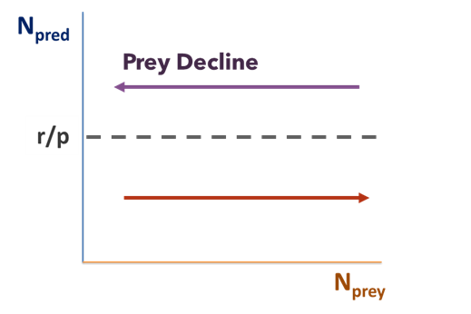
Figure \(\PageIndex{2}\): The dotted line (r/p) shows the isocline of zero growth for prey. They purple and orange lines show the direction of the prey and predator populations.
In words, the predator population reaches equilibrium when the prey population equals the predator’s starvation rate over the product of attack rate times conversion efficiency. Note that this is also a constant, and like the solution for the prey population, it does not specify the equilibrium size of the predator population, only the size of the prey population at which the predators are at equilibrium.
The isocline of Zero Growth for Predator occurs at Nprey = d/cp
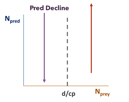
Figure \(\PageIndex{3}\): The dotted line shows the isocline of zero growth for predators (d/cp), while the purple and orange lines describe the direction the predator and prey populations will trend towards.
Now that we have solved for these isoclines, we can plot the population sizes of the two interacting populations on the two axes of a graph. The equilibrium solutions then become straight-line zero net growth isoclines (ZNGIs).
On this graph, the ZNGI for the prey population is a horizontal line at rprey/p (orange line), below which the prey population increases, and above which it decreases. The ZNGI for the predator population is a vertical line at d/cp (blue line), to the left of which the predator population decreases, and to the right of which it increases (dashed arrows).
Where the two lines cross—at the point [d/cp, rprey/p]—the two populations are at equilibrium. The continuous-time Lotka-Volterra model predicts that the point representing the two populations will cycle endlessly around the point where the two ZNGIs cross.
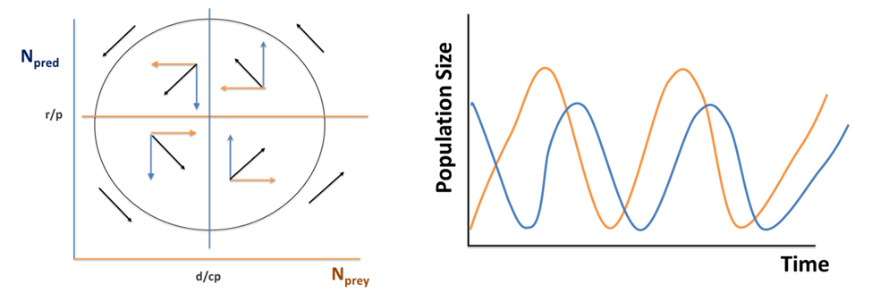
Figure \(\PageIndex{4}\): To the left, the isoclines for zero predator and prey growth are plotted. The vector arrows in each quadrant describe the counter-clockwise trends of the populations based on the movement from their initial populations to the point of equilibrium created by the isoclines. To the right, the boom-and-bust cycle of the populations are shown.
A Quick Summary - Coupled Predator-Prey Models
Based on the Exponential Model:
• Predators decline exponentially without food (prey)
• Prey increase exponentially without predation
Outcomes Depend on:
• Predator functional (p) and numerical (c) response
• Predator and prey birth/death rate
• Predator and prey initial population size
Steps for Finding the Oscillations:
• Find and plot d/cp
• Find and plot and r/p
• Plot initial population
• At isoclines, either predator or prey change trajectory