15.5: Quantifying Competition Using the Lotka-Volterra Model

 

 

Real populations do not exist in isolation, but share habitats with populations of other species. In many cases, coexisting species will interact by interspecific competition, predation, parasitism, mutualism, or other ecological interactions. More realistic models must take such interactions into account. In the 1920s, Vito Volterra and Alfred Lotka (1932) independently developed models of interspecific competition (competition between two species), and investigated the conditions that would permit competing species to coexist indefinitely. 

 

An important ecological generalization, the competitive exclusion principle, has grown out of the Lotka-Volterra model and from other sources. This principle states that two species cannot coexist unless their niches are sufficiently different that each limits its own population growth more than it limits that of the other. In other words, if there is too much niche overlap, one species will competitively exclude the other. In reality, whether two species coexist depends not only on their competitive interactions with each other, but also on their interactions with the abiotic environment and with other species not included in this simple model. Nevertheless, the competitive exclusion principle has proven fruitful in stimulating research and understanding ecological interactions in the natural world. 

 

In broad terms, the questions Lotka and Volterra asked were: 

• What will happen to the population dynamics of these two populations, given various values of the model parameters? 

• Are there parameter values that will produce a winner and a loser—one population that persists while the other goes extinct? This would be competitive exclusion. 

• Will other values result in coexistence, in which both competing populations persist indefinitely? 

 

Model Development – Starting with One Species

The logistic model of population growth focuses on intraspecific competition (competition between individuals of the same species). To keep things (relatively) simple, we will develop our model of interspecific competition beginning with this form of the logistic model:

 

\[ \frac{d N_{1}}{dt}=r_{1} N_{1}\left(\frac{K_{1}-N_{1}}{K_{1}}\right) \nonumber\]

 

where K is the carrying capacity, or largest sustainable population. The value of K is set by available resources and by each individual’s resource demand. This version of the logistic model has intraspecific competition built into it in the term (K – N_t)/K. This term reduces the population growth rate in response to the addition of each new member of the population, representing the reduction in per capita birth rate, and increase in per capita death rate, caused by competition for limited resources. 

 

The Lotka-Volterra model of interspecific competition builds on the logistic model of a single population. It begins with a separate logistic model of the population of each of the two, competing species.

 

Population 1: 

\[ \frac{d N_{1}}{dt}=r_{1} N_{1}\left(\frac{K_{1}-N_{1}}{K_{1}}\right) \nonumber\]

 

Population 2: 

\[ \frac{d N_{2}}{dt}=r_{2} N_{2}\left(\frac{K_{2}-N_{2}}{K_{2}}\right) \nonumber\]

 

Note the use of subscripts 1 and 2 to denote which species’ population is being modeled. Each population has its own rate of increase r and carrying capacity K, and these may differ between the two species.

 

Model Development – Coupling Two Competitors

Next, we build interspecific competition into each of these equations. We assume that each new member of Population 1 reduces resources available to each member of Population 2, and thus reduces population growth rate. Additionally, new members of Population 2 will also reduce resources available to members of Population 1—this is, after all, the meaning of interspecific competition.

 

The simplest way to model this would be to modify the (K₁ – N_1,t)/K term into (K₁ – N_1,t – N_2,t)/K₁. However, this assumes that each additional member of Population 2 will affect Population 1 exactly as much as an additional member of Population 1. That is not necessarily the case, so we multiply N_2,t in this term by a competition coefficient, α₁₂ to express how much effect each additional member of Population 2 has on Population 1, relative to the effect of a new member of Population 1. We modify the model for Population 2 in a parallel way. The resulting Lotka-Volterra model of two-species competition is:

 

Population 1: 

\[ \frac{d N_{1}}{dt}=r_{1} N_{1}\left(\frac{K_{1}-N_{1}-a_{12} N_{2}}{K_{1}}\right) \nonumber\]

 

Population 2: 

\[ \frac{d N_{2}}{dt}=r_{2} N_{2}\left(\frac{K_{2}-N_{2}-a_{21} N_{1}}{K_{2}}\right) \nonumber\]

 

Note the subscripts on the competition coefficients: α₁₂ expresses the effect of one member of Population 2 on the growth rate of Population 1; α₂₁ expresses the effect of one member of Population 1 on the growth rate of Population 2. 

 

The value of the competition coefficient tells us something about the relative importance of interspecific and intraspecific competition on the population dynamics of a species. 

• When the competition coefficient is less than 1, intraspecific competition has a stronger per capita impact on resource availability for that species. 

• When the competition coefficient is greater than 1, interspecific competition has a stronger per capita impact on resource availability for that species. 

• When the competition coefficient is equal to 1, inter and intraspecific competition have a similar per capita impact on resource availability for that species. 

 

Equilibrium Solutions for Coupled Competitors

To understand the outcome of competition between these two species, we must first find the equilibrium solutions to the coupled equations above. The equilibrium is the population size at which the population stops growing. We can solve for this equilibrium by setting dN/dt for each species to zero and solving for N.

 

For Population 1, for example: 

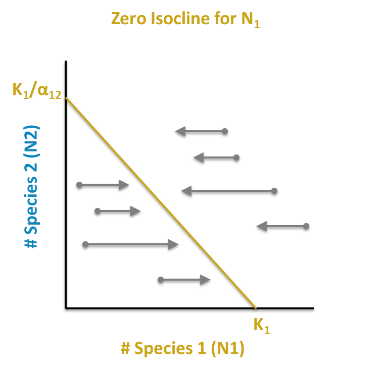
\[ \mathrm{N}_{1}=K_{1}-a_{12} N_{2} \nonumber\]

 

The resulting equation is the equation of a line, y = a + bx. We call this line a zero net growth isocline, or ZNGI, because anywhere along it, Population 1 has zero net growth. In other words, this is an equilibrium solution for Population 1. 

 

Just as x and y in the general linear equation y = a + bx can be used as coordinates for graphing, so we can use N1 and N2 as coordinates to graph each species ZNGI. We can graph this isocline by finding any two points along it and connecting them with a straight line. 

 

Two convenient points are where N_2,t = 0 and where N_1,t = 0.  If we solve for these intercepts, we wind up with the following two coordinates for Population 1: [0, K₁/a₁₂] (setting x, or the size of Population 1, to 0) and [K₁, 0] (setting y, or the population size of Population 2, to 0). In words, if there are no members of Population 2 in the habitat, Population 1 will stabilize at its own carrying capacity, K1. This seems a reasonable solution. If there are no members of Population 1, Population 2 will stabilize at the carrying capacity of Population 1 accounting for the relative per capita resource requirements of Population 2 relative to Population 1. These points can be plotted and connected to visualize the ZNGI.

 

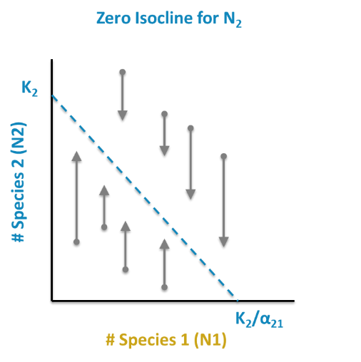
The same is done for Population 2:

\[ \mathrm{N}_{2}=K_{2}-a_{21} N_{1} \nonumber\]

 

This results in the following ZNGI coordinates: [0, K₂] and [K₂/a₂₁,0].

 

 

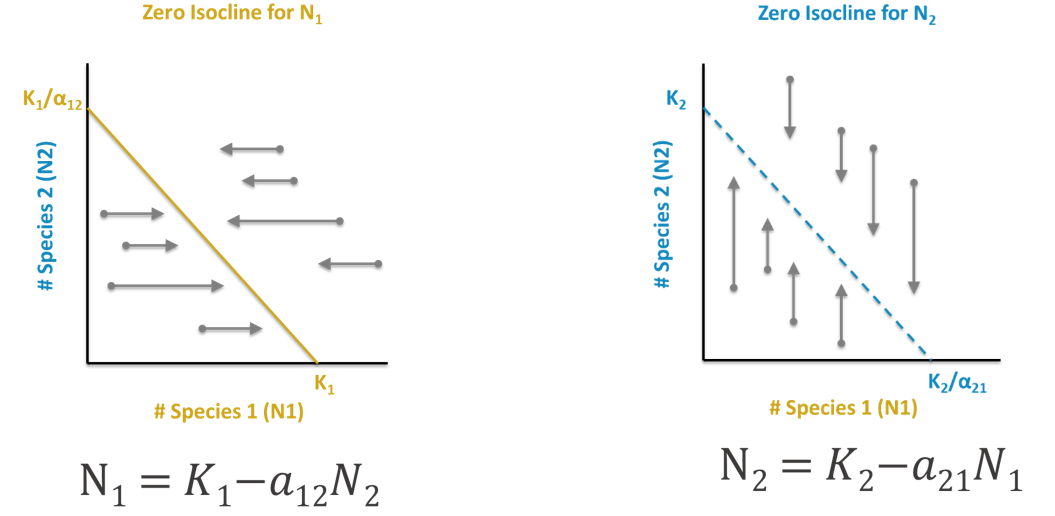
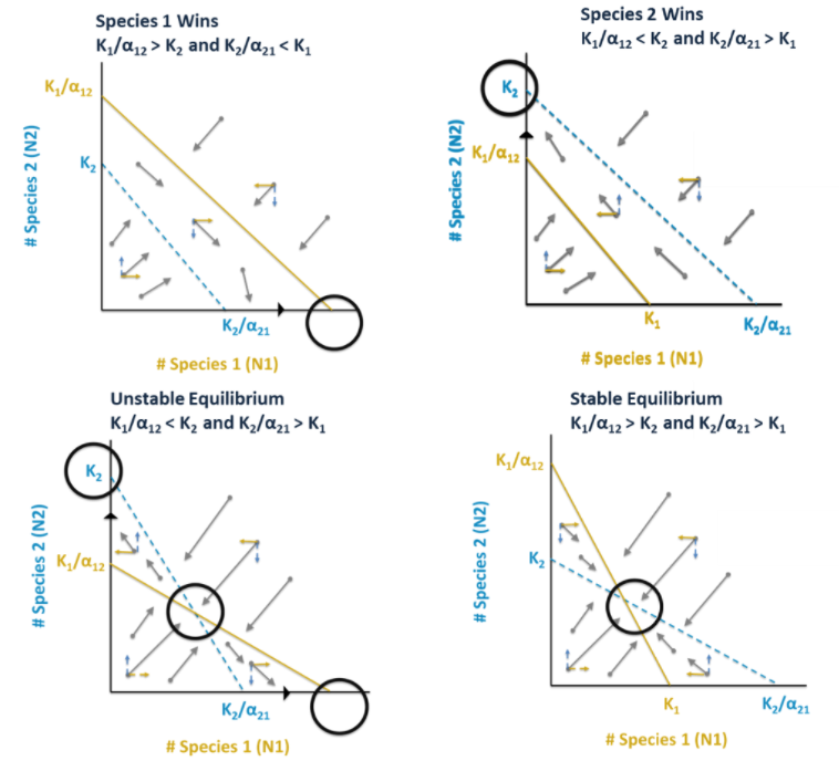
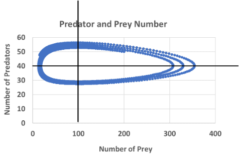
To determine the outcome of competition, we must be able to find the ZNGI lines and the initial sizes of each population and graph them. We can graph the populations of the two species at any time by a point on a graph. Population 1 should always be plotted on the x-axis and Population 2 is on the y-axis. If the point falls below (Population 1) and/or to the left (Population 2) of a species’ isocline, that population will continue to increase. If the point falls above (Population 1) and/or to the right (Population 2) of a species’ isocline, that population will decrease. This will continue to occur as the coupled populations change sizes, and the point describing the two populations will trace some trajectory across the graph, eventually reaching an equilibrium of coexistence or competition exclusion. 

 

Notice that time does not appear on either axis of this graph. The plots above are called phase diagrams, and the space bounded by its axes is called phase space. You can plot the trajectory of two changing populations through the phase space and from that determine whether one species excludes the other, or if they coexist. 

 

 

A Quick Summary of Coupled Interspecific Competition Models

 

Based on the Logistic Model:

• Alone, Species 1 and 2 increase to their K

• Species 1 and 2 reduce each others’ K

Outcomes Depend On: 

• Competition coefficient 

• Species 1 and Species 2 carrying capacity

• Species 1 and Species 2 starting population size

Steps to Determining Outcomes: 

• Find and plot Species 1 isocline (K₁ on x; K₁/α₁₂ on y)

• Find and plot Species 2 isocline (K₂/α₂₁ on x; K₂ on y)

• Plot initial population size

• Determine vectors and outcome

 

 

Models Review - Exponential, Logistic, Competition

 

Exponential (Review) – No Carrying Capacity

 

\[ \frac{d N_{1}}{dt}=r_{1} N_{1} \nonumber\]

 

r₁ = intrinsic growth rate of species 1

N₁ = population size of species 1

 

Logistic (Review) – Single Species, Carry Capacity

 

\[ \frac{d N_{1}}{dt}=r_{1} N_{1}\left(\frac{K_{1}-N_{1}}{K_{1}}\right) \nonumber\]

 

K₁ = carrying capacity of species 1 (when K = N, dN/dt = 0)

 

 

Competition – Two Species Logistic Model, Equations Linked 

Population 1: 

\[ \frac{d N_{1}}{dt}=r_{1} N_{1}\left(\frac{K_{1}-N_{1}-a_{12} N_{2}}{K_{1}}\right) \nonumber\]

 

Population 2: 

\[ \frac{d N_{2}}{dt}=r_{2} N_{2}\left(\frac{K_{2}-N_{2}-a_{21} N_{1}}{K_{2}}\right) \nonumber\]

 

α₁₂ or α = a measure of the per capita effect of species 2 on the growth of species 1

α₂₁ or β = a measure of the per capita effect of species 1 on the growth of species 2

 

 

 

Species 1 and Species 2 Isoclines

 

Species 1 and Species 2 Outcomes

 

Predator/Prey Relations Exercise \(\PageIndex{1}\)

Blue crabs have a death rate of 0.005 and an initial population size of 50. Oysters have an intrinsic growth rate of 0.1 and an initial population size of 200. For each 50 oysters a crab consumes, they can produce one additional baby blue crab. For every 400 additional oysters added to the population, each crab can consume one more oyster per unit time.

1) Where are the crab and oyster isoclines?

2) Draw a phase diagram with the isoclines. Note where the starting populations of both species are, as well as the directions of the vectors of the population changes in each quadrant.

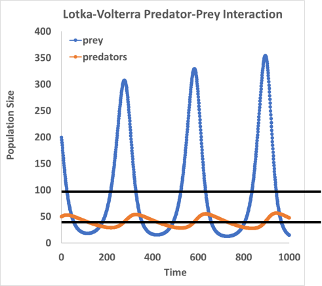
3) Draw the boom-and-bust oscillations for these species.

4) If oysters evolved to have thicker and harder to open shells, which term of the predator-prey model would be impacted, and in what direction?

5) Although the oyster population has crashed due to overfishing, the blue crab population continues to increase. What might have caused this dynamic?

6) The oyster's predators and competitors have been eradicated, but their population stops growing after a long period of increase. Why has their population stopped growing?

Answer

1) Isocline for predators (0 growth rate of predators): Nprey = d/cp = 0.005/(0.02*0.0025) = 100

Isocline for prey (0 growth rate for prey): Npred = r/p = 0.1/0.0025 = 40

2) 

3) 

4) Handing time would increase, so p would decrease.

5) Prey-switching is a possible explanation.

6) The population has reached their carrying capacity.

Phase Diagram Exercise \(\PageIndex{2}\)

Two species of monkey in West Africa, putty-nosed monkeys (Species 1) and Diana monkeys (Species 2), have nearly identical niches and breed at the same time annually. Diana monkeys eat insects and fruit, but the putty-nosed monkey eats only insects. A team of ecologists conducting a study on competition between these two species find that:

For the putty-nosed monkey population, Diana monkeys have a per capita impact equivalent to 0.8 putty-nosed monkeys.

For the Diana monkey population, putty-nosed monkeys have a per capita impact equivalent to 0.6 Diana monkeys.

Putty-nosed monkeys have a carrying capacity of 300 and starting population of 250.

Diana monkeys have a carrying capacity of 500 and starting population of 400.

1) Why does it make sense for both populations to have a competition coefficient of less than one?

2) What is a change that one of these populations could make to reduce competition?

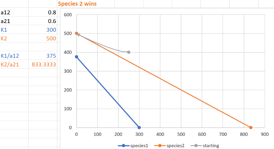
3) What are the isoclines for these competitors? Graph the isoclines. Which species wins, if any, and what is the name for this type outcome?

Answer

1) Since the two monkey species have differences in their diets, they are more likely to impact themselves than they are to impact each other—putty-nosed monkeys will not take fruit from Diana monkeys. For both species, intraspecific competition is stronger than interspecific competition.

2) One of the populations could change the time of year that they breed; the Diana monkeys can focus their diets on fruit; the populations could focus their diets on different types of insects.

3) 

References

Lotka, A.J. (1932). The growth of mixed populations: Two species competing for a common food supply. Journal of the Washington Academy of Sciences, 22, pp. 461 469.

Contributors and Attributions 

This chapter was written by N. Gownaris and T. Zallek, with text taken from the following CC-BY resources:

• Donovan, T. M. and C. Welden. 2002. Spreadsheet exercises in ecology and evolution. Sinauer Associates, Inc. Sunderland, MA, USA.