14.3: Ecosystem Monitoring

A complex and adaptive ecosystem in which all the chemical, physical, and biological components, functions, and processes are intact and functioning normally is considered a healthy ecosystem (but see Cumming and Cumming (2015), for a discussion on this value-based term). In contrast, disturbing any of an ecosystem’s components, functions, and/or processes will, by definition, alter them to some degree (Table 14.3.1). In many cases, ecosystems that have been exposed to certain forms and levels of disturbances remain healthy because there is redundancy in the roles performed by different ecosystem components. This ability of an ecosystem to withstand certain forms and levels of disturbances is referred to as ecosystem stability. Ecosystem stability could be the result of one or both of two qualities: resistance and resilience. Resistance is the ability of an ecosystem to retain the same characteristic communities and natural cycles throughout and after a disturbance event, while resilience is the ability of an ecosystem to rapidly recover or adapt after a disturbance event. For example, if the number of native aquatic insect species decline after non-native fishes are introduced to previously fish-free ponds, the pond’s ecosystem has low resistance. But if the native insect community recovers rapidly after the non-native fishes were removed, the ecosystem is resilient.

Table 14.3.1 Three ways how humans have changed the natural world.

Natural function	Changes attributed to human activities
Land surface	As much as half of the world’s ice-free land surface has been transformed to cater to people’s need for natural resources. Much of these changes are driven by agricultural activities.
Nitrogen cycle	Human activities release massive amounts of nitrogen into natural ecosystems on a daily basis. Much of this occurs through the use of nitrogen fertilisers, burning fossil fuels, and cultivating nitrogen-fixing crops.
Atmospheric carbon cycle	Scientists estimate that humans would have doubled levels of carbon dioxide in the Earth’s atmosphere by the middle of this century. This is primarily the result of fossil fuel use and deforestation.
Wildlife populations	Human activities are currently causing a sixth mass extinction.
Pollutants	Pollution from human activities have become so omnipresent that it is hard to escape its impacts. Microplastics have been found in drinking water and the food we eat.

Sources: MEA, 2005; Kulkarni et al., 2008; http://www.livingplanetindex.org

Many forms of ecosystem disturbances are easy to observe. Consequently, monitoring these visible forms of disturbances—such as the outright destruction of a forest or plastic pollution on a beach—focuses less on detection and more on developing systematic survey protocols that can provide information on whether a disturbance is spreading and increasing in intensity, or whether conservation action is successful in containing the threat. However, some disturbances are subtler, unobtrusive, and thus difficult to detect; examples include pesticide drift and agricultural runoff. Adopting a “wait and see” approach to detecting these invisible forms of disturbances can be particularly damaging, since that approach generally ends at a point where the harm will either be impossible to reverse or will require significantly more resources and time than would have been the case if the problem was addressed earlier. In this way, there are many similarities between monitoring ecosystem health and human health—some ailments are easier to diagnose than others, but we avoid the worst-case scenarios by screening regularly for diseases and treating the threatening ones promptly.

Figure 14.3.1 Biologists sampling benthic invertebrates from Lake Ontario, which straddles the New York/ Canada boundary, as part of a Cooperative Science and Monitoring Initiative project . (Photo By NYS DEC, via Flickr, CC-BY-NC-ND-2.0).

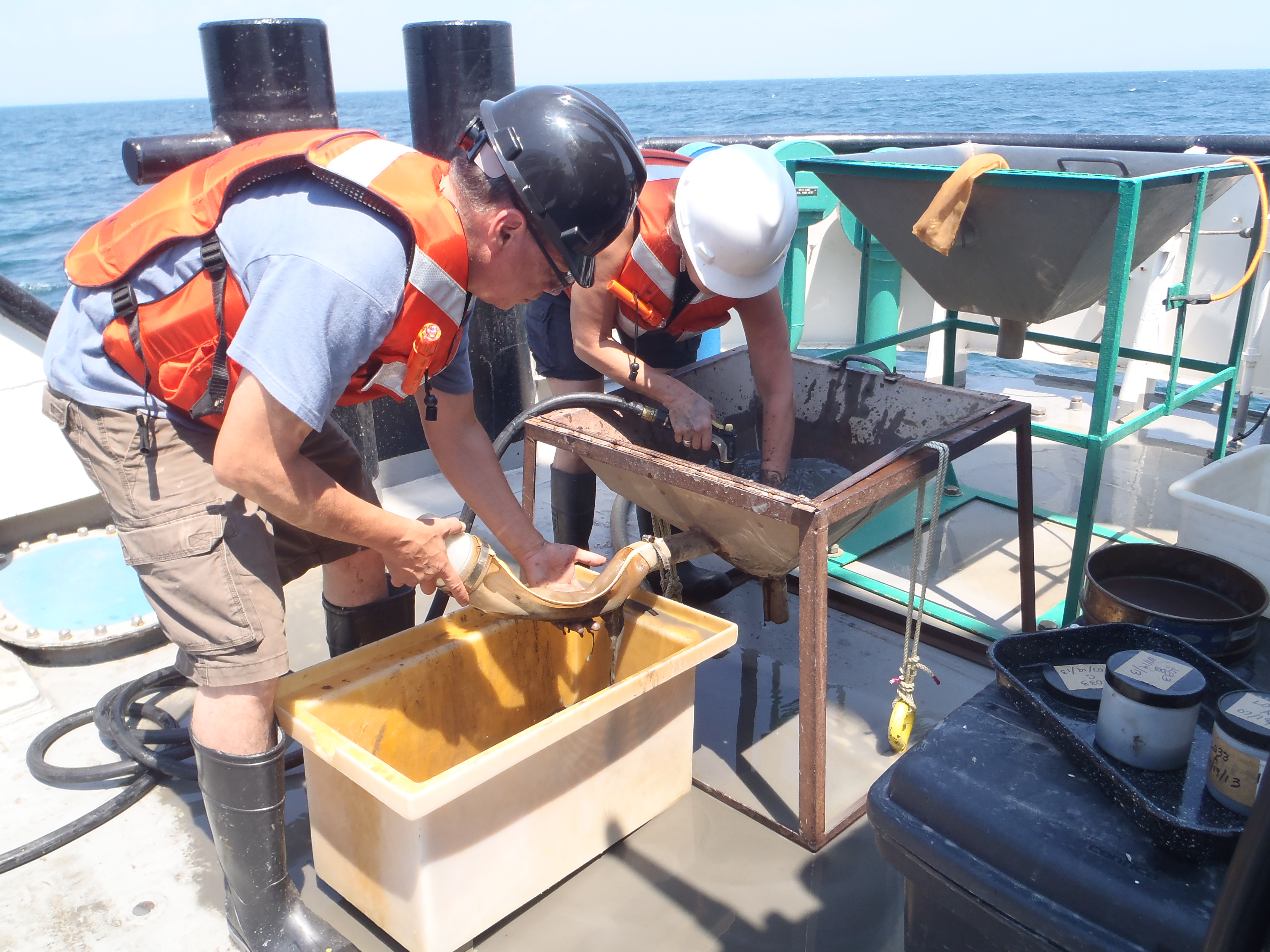
Perhaps the most popular method conservation biologists use to monitor ecosystem health is known as biomonitoring. By monitoring the abundance and/or fitness of sensitive species (Box 14.3), biologists can sometimes detect ecosystem degradation before it becomes apparent to the human eye or escalates to a point where it starts impacting human lives (Bornman and Bouwman, 2012). Monitoring environmental indicators such as macroinvertebrates (Figure 14.3.1) is particularly popular when examining the ecological condition of aquatic ecosystems; mayflies, caddisflies, and stoneflies—specialists of undisturbed streams—are often replaced by flies and midges in polluted and disturbed environments. Sometimes however, when plants or animals are not easily monitored, certain aspects of those species can still be monitored. One example is monitoring total plant biomass as a proxy for soil nutrients or intensity of herbivory. Another option is to perform a bioassay, during which a sensitive organism (typically water fleas or plankton) is released into a potentially contaminated environment to see if death or declining health occurs.

Box 14.3 Using Insects to Monitor Environmental Health

Rosina Kyerematen

Department of Animal Biology and Conservation Science,

University of Ghana, Legon, Ghana.

[e-mail]

Insects are important to nearly every terrestrial food web in the world and serve a multitude of different purposes: some insects are responsible for pollination of plants while others are scavengers that clean up dead plant and animal material. In some cases, our understanding of an insect species’ ecological role can make it suitable as an indicator of environmental health. Biomonitoring looks at the presence and abundance of organisms within their natural communities to assess the impact of environmental disturbances; this knowledge can then be used to guide ecosystem management. An indicator taxon is one whose impact can be specifically and precisely measured; its abundance serves as a measure of the overall health of an ecosystem. Understanding how the presence and abundance of indicator species, and the relative abundance of tolerant and intolerant species, reflects the relative health of an environment can allow for rapid surveys of impaired ecosystems to assess trends as well as to track changes following remediation and restoration efforts.

Over the past few years, biomonitoring with insects as indicator taxa has become increasingly popular in Ghana. Butterflies are especially popular because they show varying relative sensitivities to environmental change; the abundance of certain butterfly species can for example be used to study the impact of habitat loss, fragmentation, and climate change (Kyerematen et al., 2018). The presence and abundance of butterflies more characteristic of open and disturbed ecosystems (Figure 14.3.2) can, for example, be used as an indicator of forest degradation.

Figure 14.3.2 Because the green-banded swallowtail (Papilio nireus) prefers open woodlands, researchers in Ghana are using their abundances in forests as a measure of habitat degradation. Photograph by Celesta von Chamier, CC BY 4.0.

Aquatic insects, particularly benthic macroinvertebrates, are also useful bioindicators. Freshwater resources, such as lakes and rivers, provide water for drinking and washing to local people, and a home for economically important taxa, such as fish and shellfish. Protecting these water sources is therefore important for safeguarding people’s health and livelihoods. The presence, absence, and diversity of certain benthic macroinvertebrates, even at the order level, can provide valuable information about whether a waterbody is being degraded or not (Kyerematen et al., 2014; Nnoli et al., 2019). A recent study showed that dragonfly and damselfly diversities and populations along the coastal Densu River in Ghana vary widely depending on the physical condition of the river and surrounding area (Acquah-Lamptey et al., 2013).

With their high diversity and varying tolerances for ecosystem conditions, insects are extraordinarily suited as ecological indicators in environmental monitoring. Each insect species is also part of a wider biological community with important ecological roles. If lost, not only will an abundance of other life be affected, such a loss may also hint at a looming crisis facing people living in those compromised ecosystems.

At times, conservation biologists may need to measure the physical environment to assess environmental health. This approach is particularly common when tracking pollution, for example by monitoring for changes in biochemical indicators. For example, measuring total phosphorus, nitrogen, and dissolved oxygen load in streams and other surface water can help scientists track eutrophication. Measuring these and other biochemical indicators is usually accomplished directly via chemical analysis of environmental samples, such as soil and water. Sometimes however, biochemicals indicators are tracked indirectly via biological samples obtained from plants and animals. Because they bio-accumulate heavy metals and other pollutants, filter feeders such as clams and mussels (e.g. Bodin et al., 2013) are particularly useful in this regard as they can be used to detect very low concentrations of harmful chemicals in the environment.

Monitoring ecosystems with geospatial analysis

A persistent challenge facing biologists who monitor ecosystems—and other aspects of biodiversity—is achieving consistency across space and time. Consider a survey of a sensitive bird community to track ecosystem change; not only will different observers have varying levels of experience, but they will almost certainly see different birds during an early morning census compared to one later in the afternoon due to differences in biology and behavior between species. These factors introduce error into monitoring data, which in turn can mask the effect a biologist tries to measure (Buckland and Johnston, 2017). Laboratory scientists’ control for these confounding factors by making multiple measurements under strictly controlled conditions. But for conservation biologists working outside in the wind and rain, repeated observations under similar conditions can be near impossible.

Geospatial analysis offers a variety of tools that allow biologists to overcome some of these traditional field monitoring challenges. These tools use geographic information systems (GIS) computer software packages to store, display, and manipulate a wide variety of data representing the natural environment, biodiversity, and human land-use patterns as they relate to one another on Earth’s surface. GIS thereby allows biologists to easily visualize and analyze spatial relationships between mapped data, which may include aspects such as vegetation types, climate, soils, topography, geology, water availability, species distributions, existing protected areas, human settlements, and human resource use (Figure 14.3.3). Understanding such relationships helps conservation biologists to prioritize their actions, for example by identifying areas where data are lacking, where an environmental change requires further investigation, or where gaps in regional protected areas network exist.

Figure 14.3.3 Distribution maps for three threatened species are overlaid onto maps of protected areas and vegetation types to identify potential conservation gaps. This GIS analysis shows that Species A is well protected, Species B is protected to some extent, and Species C is not protected at all. Species C would thus be considered a high conservation priority. After Scott et al., 1991, CC BY 4.0.

Remote sensing is a special branch of geospatial analysis directed at obtaining ecosystem data without making physical contact (i.e. boots on the ground) with the observation site. Before the turn of the 20th century, the most popular form of remote sensing was aerial photography from airplanes. These aerial photographs facilitated geographers’ ability to draw maps of landscape features, including human infrastructure and natural vegetation patterns. Remote sensing opportunities greatly expanded from 1960 onward, with the launch of the National Aeronautical Space Administration’s (NASA) first Earth observation satellites, to take photographs of Earth from space for weather forecasting. Subsequent satellite programs expanded their scope to also collect additional data of Earth’s surface and atmosphere. While much of this data would have been useful to conservation, early satellite data products were very expensive and thus largely out of reach of the larger conservation community. This all changed in 2008 when NASA started distributing their Earth observation products for free to the public, heralding an era in which remote sensing became a standard tool in the conservation field.

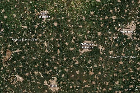
Today, hundreds of Earth observation satellites circle the planet, offering near real-time access to unbiased and consistent environmental datasets of nearly all terrestrial surfaces, oceanic surfaces and floor depths, and the atmosphere, all from the comfort of a computer connected to the internet (Wilson et al., 2013). Scientists use these products in ecosystem monitoring efforts, including monitoring water quality (Dube et al. 2015), forest loss (Laporte et al., 2007) (Figure 14.3.4), coral reef health (McClanahan et al., 2011), desertification (Symeonakis et al., 2004), and fire regimes (Archbald et al., 2010). Linking the information obtained by Earth observation satellites to biological information collected on the ground has proved invaluable in monitoring species’ threat statuses (Di Marco et al., 2014), ecosystem connectivity (Wegmann et al., 2014), and habitat suitability (Torres et al., 2010), as well as understanding how biodiversity responds to environmental changes.

Figure 14.3.4: NASA's Landsat images of the Nile Delta from 1984 (left) to 2021 (right). Egypt is losing agricultural land in the Nile Delta due to urban development at an alarming rate. Only 4% of Egypt's land is suitable for agriculture and is being converted as the population in Egypt has grown to 100 million, of which 95% live in the Nile Delta. (Image courtesy of NASA)

The popularity and utility of these products have preceded and facilitated the expansion of other remote sensing applications in ecosystem monitoring. Among the most popular are radar products (Figure 14.3.5), which have become the standard method for obtaining elevation and other terrain data (NASA, 2009, 2013), as well as estimates of carbon stocks (Carreiras et al., 2012). Advances have also been made in using hyper-spectral imagery to monitor soil properties (Mashimbye et al., 2012) and even individual trees (Naidoo et al., 2012). LiDAR has enabled biologists to map three-dimensional vegetation, which can be used to explain animal movements (Loarie et al., 2013; Davies et al., 2016) and measure carbon stocks and forest loss (Burton et al., 2017).

Figure 10.3.5 A radar composite of equatorial Africa obtained in 1996 by Japan’s Earth Resources Satellite. The area shown covers about 7.4 million km2. Due to the filters applied to the image, yellow represents flooded forests, palm plantations, and urban areas; green represents forest, and black represents surface water. Savannahs may be black, blue, purple, or green, depending on the ecoregion type. Displays such as these allow researchers to map ecosystems, and ecosystem loss at a much larger scale than if only field observations were used. Image courtesy of NASA, https://images.nasa.gov/details-PIA01348.html, CC0.

Despite the opportunities presented by remote sensing, it is critical to remember that it is not a substitute for traditional field monitoring methods. Most importantly, remote sensing applications cannot be considered reliable without verification using field data (see Burton et al., 2017). Most remote sensing products are also relatively new, which does not allow for enough opportunities to compare across time. In the absence of historical remotely sensed data, geospatial analysts usually choose the best reference site currently available; this may expose those analysts to shifting baseline syndrome, because the chosen reference site may be vastly different from earlier states the scientists are actually interested in studying (Bunce et al., 2008; Papworth et al., 2009). Remote sensing is, therefore, not a cure-all for ecosystem monitoring challenges; it is simply a powerful tool to supplement traditional field-based monitoring.