8.10: Chapter 8 Answers

Chapter 8 Answers

1. 1. 1. 1. case 1 – co-dominance
         2. case 2 – incomplete-dominance (partial-dominance)
         3. case 3 – incomplete penetrance
         4. case 4 – pleiotropy
         5. case 5 – haplo-sufficiency of the A2 allele for white phenotype
         6. case 6 – haplo-insufficiency of the A2 allele for white phenotype
         7. case 7 – broad (variable) expressivity of A2 allele
      2. If 1 and 2 and 3 are all colorless, and 4 is red, what will be the phenotypes associated with the following genotypes? All of these mutations are recessive. As always, if the genotype for a particular gene is not listed, you can assume that alleles for that gene are wild-type.
         1. red (because A and B are redundant, so products 3 and then 4 can be made)
         2. red (because A and B are redundant, so products 3 and then 4 can be made)
         3. white (because product 3 will accumulate and it is colorless)
         4. white (because only product 1 and 2 will be present and both are colorless)
         5. white (because only product 1 and 3 will be present and both are colorless)
         6. white (because only product 2 and 3 will be present and both are colorless)
         7. white (because only product 1 and 2 will be present and both are colorless)
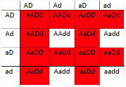
         8. 15 red : 1 white
            
         9. 12 red: 4 white
            
         10. 12 red: 4 white
             
      3. 1. red (because A and B are redundant, so products 3 and then 4 can be made)
         2. red (because A and B are redundant, so products 3 and then 4 can be made)
         3. blue (because product 3 will accumulate, and it is blue)
         4. white (because only product 1 and 2 will be present and both are colorless)
         5. blue (because only product 1 and 3 will be present and 1 is colorless and 3 is blue)
         6. blue (because only product 2 and 3 will be present and 2 is colorless and 3 is blue)
         7. white (because only product 1 and 2 will be present and both are colorless)
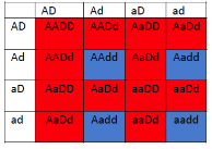
         8. 15 red : 1 white
            
         9. 12 red : 4 blue
            
         10. 12 red : 4 blue
             
      4. 1. red (because A and B are redundant, so products 3 and then 4 can be made)
         2. red (because A and B are redundant, so products 3 and then 4 can be made)
         3. blue (because product 3 will accumulate, and it is blue)
         4. yellow (because only product 1 and 2 will be present and 1 is colorless and 2 is yellow)
         5. blue (because only product 1 and 3 will be present and 1 is colorless and 3 is blue)
         6. green? (because only product 2 and 3 will be present and 2 is yellow and 3 is blue, so probably the fruit will be some combination of those two colors)
         7. yellow (because only product 1 and 2 will be present and 1 is colorless and 2 is yellow)
         8. 15 red: 1 yellow
            
         9. 12 red: 3 blue:1 green
            
         10. 12 red: 4 blue
             
      5. Epistasis is demonstrated when the phenotype for a mutant in one locus is prevented from being expressed by a mutant at another locus. In this case, we would expect a homozygous mutant at one locus (e.g., D) to be the same phenotype as a homozygous mutant in both loci (e.g., D and A, or D and B).
         So, the following situations from questions 2-4 demonstrated epistasis: Q#2: No epistasis can be determined from the phenotypes (even though we know from the pathway provided that D is downstream of A and B). There are only two possible phenotypes. So even though the D locus might be epistatic to A and B, one cannot see this interaction because the product of both A and B (compound 3) is colourless.
         Q#3: The phenotypes show that D is epistatic to A and B:
         • aadd looks like AAdd or Aadd; dd prevents the expression of the A or a alleles.
         • bbdd looks like BBdd or Bbdd: dd prevents the expression of the B or b alleles.

         Note: that the triple mutant aabbdd would be colourless (white).
         Q#4: The phenotypes show that D is epistatic to A, because aadd looks like AAdd or Aadd.
         With bbdd, the difference between bbdd (green), Bbdd (blue), and BBdd (blue) is apparent, Thus, the phenotypes do not provide evidence for epistasis between B and D.

      6. The answer is the same for a→d
         • P could have been either: AABB × aabb or aaBB × AAbb;
         • F1 was: AaBb × AaBb
         • Conduct an enhancer/suppressor screen (which can also result in the identification of revertants, as well)

         Allow the plants to self‐pollinate in order to make any new, recessive mutations homozygous.

      7. Depending which amino acids were altered, and how they were altered, a second mutation in g*g* could either have no effect (in which case the phenotype would be the same as gg), or it could possibly cause a reversion of the phenotype to wild‐type, so that g*g* and GG have the same phenotype.
      8. Depending on the normal function of gene A, and which amino acids were altered in allele a, there are many potential phenotypes for aagg.
         Case 1: If the normal function of gene A is in an unrelated process (e.g., A is required for root development, but not the development of leaves), then the phenotype of aagg will be: short roots and narrow leaves. The phenotypic ratios among the progeny of a dihybrid cross will be:

         9	3	3	1
         A_G_	A_gg	aaG_	aagg
         wild-type	tubular leaves normal roots	short roots normal leaves	tubular leaves short roots

         Case 2: If the normal function of gene A is in the same process as G, such that a is a recessive allele that increases the severity of the gg mutant (i.e., a is an enhancer of g) then the phenotype of aagg could be : no leaves. The phenotypic ratios among the progeny of a dihybrid cross depend on whether aa mutants have a phenotype independent of gg, in other words, do aaG_ plants have a phenotype that is different from wild‐type or from A_gg. There is no way to know this without doing the experiment, since it depends on the biology of the particular gene, mutation and pathway involved.

         The following (2a, 2b, 2c) are the three possible outcomes:

         Case 2a) If aa is an enhancer of gg, and aaG_ plants have a mutant phenotype that differs from wild‐type or (A_gg) then the phenotypic ratios among the progeny of a dihybrid cross will be:

         9	3	3	1
         A_G_	A_gg	aaG_	aagg
         wild-type	tubular leaves (some phenotype that differs from gg; maybe small twisted leaves)	abnormal leaves	no leaves

         Case 2b) If aa is an enhancer of gg, and aaG_ plants have a mutant phenotype that is the same as A_gg , the phenotypic ratios among the progeny of a dihybrid cross will be:

         9	6	1
         A_G_	A_gg aaG_	aagg
         wild-type	tubular leaves	no leaves

         Case 2c) If aa is an enhancer of gg, and aaG_ do not have a phenotype that differs from wild‐type then the phenotypic ratios among the progeny of a dihybrid cross will be:

         12	3	1
         A_G_ aaG_	A_gg	aagg
         wild-type	tubular leaves	no leaves

         Case 3: If the normal function of gene A is in the same process as G, such that a is a recessive allele that decreases the severity of the gg mutant (i.e., a is an suppressor of g) then the phenotype of aagg could be: wild‐type. The phenotypic ratios among the progeny of a dihybrid cross depend on whether aa mutants have a phenotype independent of gg, in other words, do aaG_ plants have a phenotype that is different from wild‐type or from A_gg. There is no way to know this without doing the experiment, since it depends on the biology of the particular gene, mutation and pathway involved.
         The following (3a, 3b, 3c) are the three possible outcomes:
         Case 3 a) If aa is a suppressor of gg, and aaG_ plants have a mutant phenotype that differs from wild‐type or (A_gg) then the phenotypic ratios among the progeny of a dihybrid cross will be:

         10	3	3
         A_G_ aagg	A_gg	aaG_
         wild-type	tubular leaves (some phenotype that differs from gg)	no leaves

         Case 3 b) If aa is an suppressor of gg, and aaG_ plants have a mutant phenotype that is the same as A_gg the phenotypic ratios among the progeny of a dihybrid cross will be:

         10	6
         A_G_ aagg	A_gg aaG_
         wild-type	tubular leaves

         Case 3 c) If aa is an suppressor of gg, and aaG_ plants do not have a phenotype that differs from wild‐type then the phenotypic ratios among the progeny of a dihybrid cross will be:

         13	3
         A_G_ aaG_ aagg	A_gg
         wild-type	tubular leaves

         Case 4: If the normal function of gene A is in the same process as G, such that a is a recessive allele that with a phenotype that is epistatic to the gg mutant then the phenotype of both aaG_ and aagg could be : no leaves. The phenotypic ratios among the progeny of a dihybrid cross will be:

         9	4	3
         A_G_	aaG_ aagg	A_gg
         wild-type	no leaves	tubular leaves

      9. Closing Statement: There are many more phenotypes and ratios that could be imagined (e.g., different types of dominance relationships, different types of epistasis, lethality…etc). Isn’t genetics wonderful? It is sometimes shocking that more people don’t want to become geneticists.
      10. The point of this exercise is to show that many different ratios can be generated, depending on the biology of the genes involved. On an exam, you could be asked to calculate the ratio, given particular biological parameters. So, this exercise is also meant to demonstrate that it is better to learn how to calculate ratios than just trying to memorize which ratios match which parameters. In a real genetic screen, you would observe the ratios, and then try to deduce something about the biology from those ratios.
      11. For a dihybrid cross, there are 4 classes, 9:3:3:1. In a trihybrid cross without gene interactions, each of these 4 classes will be further split into a 3:1 ratio based on the phenotype at the third locus. For example, 9 × 3 =27 and 9 × 1 = 9. This explains the first two terms of the complete ratio: 27:9:9:9:3:3:3:1.