11.4: Fitting birth-death models to branching times
- Page ID
- 21645

\( \newcommand{\vecs}[1]{\overset { \scriptstyle \rightharpoonup} {\mathbf{#1}} } \)
\( \newcommand{\vecd}[1]{\overset{-\!-\!\rightharpoonup}{\vphantom{a}\smash {#1}}} \)
\( \newcommand{\dsum}{\displaystyle\sum\limits} \)
\( \newcommand{\dint}{\displaystyle\int\limits} \)
\( \newcommand{\dlim}{\displaystyle\lim\limits} \)
\( \newcommand{\id}{\mathrm{id}}\) \( \newcommand{\Span}{\mathrm{span}}\)
( \newcommand{\kernel}{\mathrm{null}\,}\) \( \newcommand{\range}{\mathrm{range}\,}\)
\( \newcommand{\RealPart}{\mathrm{Re}}\) \( \newcommand{\ImaginaryPart}{\mathrm{Im}}\)
\( \newcommand{\Argument}{\mathrm{Arg}}\) \( \newcommand{\norm}[1]{\| #1 \|}\)
\( \newcommand{\inner}[2]{\langle #1, #2 \rangle}\)
\( \newcommand{\Span}{\mathrm{span}}\)
\( \newcommand{\id}{\mathrm{id}}\)
\( \newcommand{\Span}{\mathrm{span}}\)
\( \newcommand{\kernel}{\mathrm{null}\,}\)
\( \newcommand{\range}{\mathrm{range}\,}\)
\( \newcommand{\RealPart}{\mathrm{Re}}\)
\( \newcommand{\ImaginaryPart}{\mathrm{Im}}\)
\( \newcommand{\Argument}{\mathrm{Arg}}\)
\( \newcommand{\norm}[1]{\| #1 \|}\)
\( \newcommand{\inner}[2]{\langle #1, #2 \rangle}\)
\( \newcommand{\Span}{\mathrm{span}}\) \( \newcommand{\AA}{\unicode[.8,0]{x212B}}\)
\( \newcommand{\vectorA}[1]{\vec{#1}} % arrow\)
\( \newcommand{\vectorAt}[1]{\vec{\text{#1}}} % arrow\)
\( \newcommand{\vectorB}[1]{\overset { \scriptstyle \rightharpoonup} {\mathbf{#1}} } \)
\( \newcommand{\vectorC}[1]{\textbf{#1}} \)
\( \newcommand{\vectorD}[1]{\overrightarrow{#1}} \)
\( \newcommand{\vectorDt}[1]{\overrightarrow{\text{#1}}} \)
\( \newcommand{\vectE}[1]{\overset{-\!-\!\rightharpoonup}{\vphantom{a}\smash{\mathbf {#1}}}} \)
\( \newcommand{\vecs}[1]{\overset { \scriptstyle \rightharpoonup} {\mathbf{#1}} } \)
\(\newcommand{\longvect}{\overrightarrow}\)
\( \newcommand{\vecd}[1]{\overset{-\!-\!\rightharpoonup}{\vphantom{a}\smash {#1}}} \)
\(\newcommand{\avec}{\mathbf a}\) \(\newcommand{\bvec}{\mathbf b}\) \(\newcommand{\cvec}{\mathbf c}\) \(\newcommand{\dvec}{\mathbf d}\) \(\newcommand{\dtil}{\widetilde{\mathbf d}}\) \(\newcommand{\evec}{\mathbf e}\) \(\newcommand{\fvec}{\mathbf f}\) \(\newcommand{\nvec}{\mathbf n}\) \(\newcommand{\pvec}{\mathbf p}\) \(\newcommand{\qvec}{\mathbf q}\) \(\newcommand{\svec}{\mathbf s}\) \(\newcommand{\tvec}{\mathbf t}\) \(\newcommand{\uvec}{\mathbf u}\) \(\newcommand{\vvec}{\mathbf v}\) \(\newcommand{\wvec}{\mathbf w}\) \(\newcommand{\xvec}{\mathbf x}\) \(\newcommand{\yvec}{\mathbf y}\) \(\newcommand{\zvec}{\mathbf z}\) \(\newcommand{\rvec}{\mathbf r}\) \(\newcommand{\mvec}{\mathbf m}\) \(\newcommand{\zerovec}{\mathbf 0}\) \(\newcommand{\onevec}{\mathbf 1}\) \(\newcommand{\real}{\mathbb R}\) \(\newcommand{\twovec}[2]{\left[\begin{array}{r}#1 \\ #2 \end{array}\right]}\) \(\newcommand{\ctwovec}[2]{\left[\begin{array}{c}#1 \\ #2 \end{array}\right]}\) \(\newcommand{\threevec}[3]{\left[\begin{array}{r}#1 \\ #2 \\ #3 \end{array}\right]}\) \(\newcommand{\cthreevec}[3]{\left[\begin{array}{c}#1 \\ #2 \\ #3 \end{array}\right]}\) \(\newcommand{\fourvec}[4]{\left[\begin{array}{r}#1 \\ #2 \\ #3 \\ #4 \end{array}\right]}\) \(\newcommand{\cfourvec}[4]{\left[\begin{array}{c}#1 \\ #2 \\ #3 \\ #4 \end{array}\right]}\) \(\newcommand{\fivevec}[5]{\left[\begin{array}{r}#1 \\ #2 \\ #3 \\ #4 \\ #5 \\ \end{array}\right]}\) \(\newcommand{\cfivevec}[5]{\left[\begin{array}{c}#1 \\ #2 \\ #3 \\ #4 \\ #5 \\ \end{array}\right]}\) \(\newcommand{\mattwo}[4]{\left[\begin{array}{rr}#1 \amp #2 \\ #3 \amp #4 \\ \end{array}\right]}\) \(\newcommand{\laspan}[1]{\text{Span}\{#1\}}\) \(\newcommand{\bcal}{\cal B}\) \(\newcommand{\ccal}{\cal C}\) \(\newcommand{\scal}{\cal S}\) \(\newcommand{\wcal}{\cal W}\) \(\newcommand{\ecal}{\cal E}\) \(\newcommand{\coords}[2]{\left\{#1\right\}_{#2}}\) \(\newcommand{\gray}[1]{\color{gray}{#1}}\) \(\newcommand{\lgray}[1]{\color{lightgray}{#1}}\) \(\newcommand{\rank}{\operatorname{rank}}\) \(\newcommand{\row}{\text{Row}}\) \(\newcommand{\col}{\text{Col}}\) \(\renewcommand{\row}{\text{Row}}\) \(\newcommand{\nul}{\text{Nul}}\) \(\newcommand{\var}{\text{Var}}\) \(\newcommand{\corr}{\text{corr}}\) \(\newcommand{\len}[1]{\left|#1\right|}\) \(\newcommand{\bbar}{\overline{\bvec}}\) \(\newcommand{\bhat}{\widehat{\bvec}}\) \(\newcommand{\bperp}{\bvec^\perp}\) \(\newcommand{\xhat}{\widehat{\xvec}}\) \(\newcommand{\vhat}{\widehat{\vvec}}\) \(\newcommand{\uhat}{\widehat{\uvec}}\) \(\newcommand{\what}{\widehat{\wvec}}\) \(\newcommand{\Sighat}{\widehat{\Sigma}}\) \(\newcommand{\lt}{<}\) \(\newcommand{\gt}{>}\) \(\newcommand{\amp}{&}\) \(\definecolor{fillinmathshade}{gray}{0.9}\)Another approach that uses more of the information in a phylogenetic tree involves fitting birth-death models to the distribution of branching times. This approach traces all the way back to Yule (1925), who first applied stochastic process models to the growth of phylogenetic trees. More recently, a series of papers by Raup and colleagues (Raup et al. 1973; Raup and Gould 1974; Gould et al. 1977; Raup 1985) spurred modern approaches to quantitative macroevolution by simulating random clades, then demonstrating how variable such clades grown under simple birth-death models can be.
Most modern approaches to fitting birth-death models to phylogenetic trees use the intervals between speciation events on a tree - the "waiting times" between successive speciation - to estimate the parameters of birth-death models. Figure 10.2 shows these waiting times. Frequently, information about the pattern of species accumulation in a phylogenetic tree is summarized by a lineage-through-time (LTT) plot, which is a plot of the number of lineages in a tree against time (see Figure 10.9). As I introduced in Chapter 10, the y-axis of LTT plots is log-transformed, so that the expected pattern under a constant-rate pure-birth model is a straight line. Note also that LTT plots ignore the relative order of speciation events. Stadler (2013b) calls models justifying such an approach "species-exchangable" models - we can change the identity of species at any time point without changing the expected behavior of the model. Because of this, approaches to understanding birth-death models based on branching times are different from - and complementary to - approaches based on tree topology, like tree balance.
As discussed in the previous chapter, even though we often have no information about extinct species in a clade, we can still (in theory) infer the presence of extinction from an LTT plot. The signal of extinction is an excess of young lineages, which is seen as the "pull of the recent" in our LTT plots (Figure 10.10). In the next chapter, I will demonstrate how statistical approaches can capture this pattern in a more rigorous way.
Section 11.4a: Likelihood of waiting times under a birth-death model
In order to use ML and Bayesian methods for estimating the parameters of birth-death models from comparative data, we need to write down the likelihoods of the waiting times between speciation events in a tree. There is a little bit of variation in notation in the literature, so I will follow Stadler (2013b) and Maddison et al. (2007), among others, to maintain consistency. We will assume that the clade begins at time t1 with a pair of species. Most analyses follow this convention, and condition the process as starting at the time t1, representing the node at the root of the tree. This makes sense because we rarely have information on the stem age of our clade. We will also condition on both of these initial lineages surviving to the present day, as this is a requirement to obtain a tree with this crown age (e.g. Stadler 2013a equation 5).
Speciation and extinction events occur at various times, and the process ends at time 0 when the clade has n extant species - that is, we measure time backwards from the present day. Extinction will result in species that do not extend all the way to time 0. For now, we will assume that we only have data on extant species. We will refer to the phylogenetic tree that shows branching times leading to the extant species as the reconstructed tree (Nee et al. 1994). For a reconstructed tree with n species, there are n − 1 speciation times, which we will denote as t1, t2, t3, ..., tn − 1. The leaves of our ultrametric tree all terminate at time 0.
Note that in this notation, t1 > t2 > … > tn − 1 > 0, that is, our speciation times are measured backwards from the tips, and as we increase the index the times are constantly decreasing [this is an important notational difference between Stadler (2013a), used here, and Nee (1994 and others), the latter of which considers the time intervals between speciation events, e.g. t1 − t2 in our notation]. For now, we will assume complete sampling; that is, all n species alive at the present day are represented in the tree.
We will now derive a likelihood of of observing the set of speciation times t1, t2, ..., tn − 1 given the extant diversity of the clade, n, and our birth-death model parameters λ and μ. To do this, we will follow very closely an approach based on differential equations introduced by Maddison et al. (2007).
The general idea is that we will assign values to these probabilities at the tips of the tree, and then define a set of rules to update them as we flow back through the tree from the tips to the root. When we arrive at the root of the tree, we will have the probability of observing the actual tree given our model - that is, the likelihood. This is another pruning algorithm.
To begin with, we need to keep track of two probabilities: DN(t), the probability that a lineage at some time t in the past will evolve into the extant clade N as observed today; and E(t), the probability that a lineage at some time t will go completely extinct and leave no descendants at the present day. (Later, we will redefine E(t) so that it includes the possibility that the lineages has descendants but none have been sampled in our data). We then apply these probabilities to the tree using three main ideas (Figure 11.4)
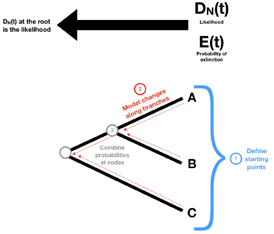
- We define our starting points at the tips of the tree.
- We define how the probabilities defined in (1) change as we move backwards along branches of the tree.
- We define what happens to our probabilities at the tree nodes.
Then, starting at the tips of the tree, we make our way to the root. At each tip, we have a starting value for both DN(t) and E(t). We move backwards along the branches of the tree, updating both probabilities as we go using step 2. When two branches come togther at a node, we combine those probabilities using step 3.
In this way, we walk through the tree, starting with the tips and passing over every branch and node (Figure 11.4). When we get to the root we will have DN(troot), which is the full likelihood that we want.
You might wonder why we need to calculate both DN(t) and E(t) if the likelihood is captured by DN(t) at the root. The reason is that the probability of observing a tree is dependent on these extinction probabilities calculated back through time. We need to keep track of E(t) to know about DN(t) and how it changes. You will see below that E(t) appears directly in our differential equations for DN(t).
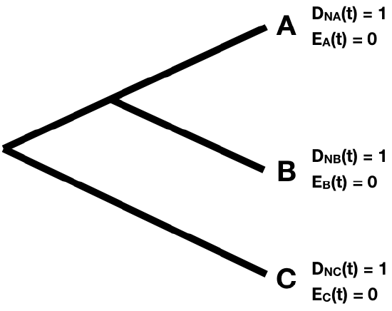
First, the starting point. Since every tip i represents a living lineage, we know it is alive at the present day - so we can define DN(t)=1. We also know that it will not go extinct before being included in the tree, so E(t)=0. This gives our starting values for the two probabilities at each tip in the tree (Figure 11.5).
Next, imagine we move backwards along some section of a tree branch with no nodes. We will consider an arbitrary branch of the tree. Since we are going back in time, we will start at some node in the tree N, which occurs at a time tN, and denote the time going back into the past as t (Figure 11.6).
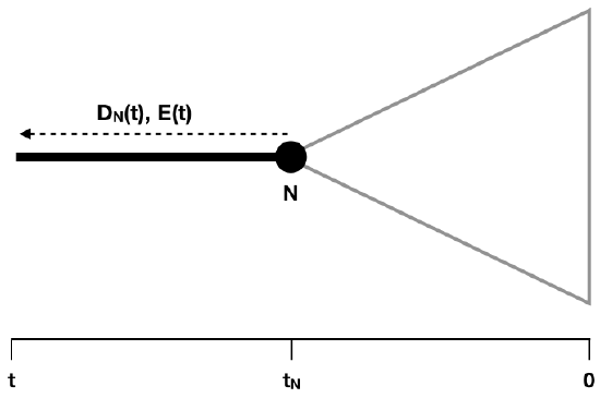
Since that section of branch exists in our tree, we know two things: the lineage did not go extinct during that time, and if speciation occurred, the lineage that split off did not survive to the present day. We can capture these two possibilities in a differential equation that considers how our overall likelihood changes over some very small unit of time (Maddison et al. 2007).
\[ \frac{dD_N(t)}{dt} = -(\lambda + \mu) D_N(t) + 2 \lambda E(t) D_N(t) \label{11.12} \]
Here, the first part of the equation, −(λ + μ)DN(t), represents the probability of not speciating nor going extinct, while the second part, 2λE(t)DN(t), represents the probability of speciation followed by the ultimate extinction of one of the two daughter lineages. The 2 in this equation appears because we must account for the fact that, following speciation from an ancestor to daughters A and B, we would see the same pattern no matter which of the two descendants survived to the present.
We also need to calculate our extinction probability going back through the tree (Maddison et al. 2007):
\[ \frac{dE(t)}{dt} = \mu - (\mu + \lambda) E(t) + \lambda E(t)^2 \label{11.13} \]
The three parts of this equation represent the three ways a lineage might not make it to the present day: either it goes extinct during the interval being considered ( μ), it survives that interval but goes extinct some time later ( −(μ + λ)E(t)), or it speciates in the interval but both descendants go extinct before the present day ( λE(t)2) (Maddison et al. 2007). Unlike the DN(t) term, this probability depends only on time and not the topological structure of the tree.
We will also specify that λ > μ; it is possible to relax that assumption, but it makes the solution more complicated.
We can solve these equations so that we will be able to update the probability moving backwards along any branch of the tree with length t. First, solving equation 11.13 and using our initial condition E(0) = 0:
\[ E(t) = 1 - \frac{\lambda-\mu}{\lambda - (\lambda-\mu)e^{(\lambda - \mu)t}} \label{11.14} \]
We can now substitute this expression for E(t) into Equation \ref{11.12} and solve
\[ D_N(t) = e^{-(\lambda - \mu)(t - t_N)} \frac{(\lambda - (\lambda-\mu)e^{(\lambda - \mu)t_N})^2}{(\lambda - (\lambda-\mu)e^{(\lambda - \mu)t})^2} \cdot D_N(t_N) \label{11.15}\]
Remember that tN is the depth (measured from the present day) of node N (Figure 11.6).
Finally, we need to consider what happens when two branches come together at a node. Since there is a node, we know there has been a speciation event. We multiply the probability calculations flowing down each branch by the probability of a speciation event [Maddison et al. (2007); Figure 11.7].
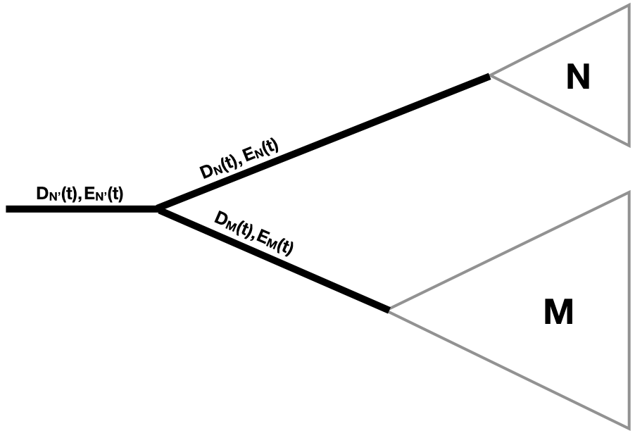
So:
\[D_{N′}(t)=D_N(t)D_M(t)λ \label{11.16}\]
Where clade N' is the clade made up of the combination of two sister clades N and M.
To apply this approach across an entire phylogenetic tree, we multiply Equations \ref{11.15} and \ref{11.16} across all branches and nodes in the tree. Thus, the full likelihood is (Maddison et al. 2007; Morlon et al. 2011):
\[ L(t_1, t_2, \dots, t_n) = \lambda^{n-1} \big[ \prod_{k = 1}^{2n-2} e^{(\lambda-\mu)(t_{k,b} - t_{k,t})} \cdot \frac{(\lambda - (\lambda-\mu)e^{(\lambda - \mu)t_{k,t}})^2}{(\lambda - (\lambda-\mu)e^{(\lambda - \mu)t_{k,b}})^2} \big] \label{11.17}\]
Here, n is the number of tips in the tree (note that the original derivation in Maddison uses n as the number of nodes, but I have changed it for consistency with the rest of the book).
The product in Equation \ref{11.17} is taken over all 2n − 2 branches in the tree. Each branch k has two times associated with it, one towards the base of the tree, tk, b, and one towards the tips, tk, t.
Most methods fitting birth-death models to trees condition on the existence of a tree - that is, conditioning on the fact that the whole process did not go extinct before the present day, and the speciation event from the root node led to two surviving lineages. To do this conditioning, we divide Equation \ref{11.17} by λ[1 − E(troot)]2 (Morlon et al. 2011; Stadler 2013a).
Additionally, likelihoods for birth-death waiting times, for example those in the original derivation by Nee, include an additional term, (n − 1)!. This is because there are (n − 1)! possible topologies for any set of n − 1 waiting times, all equally likely. Since this term is constant for a given tree size n, then leaving it out has no influence on the relative likelihoods of different parameter values - but it is necessary to know about this multiplier if comparing likelihoods across different models for model selection, or comparing the output of different programs (Stadler 2013a).
Accounting for these two factors, the full likelihood is:
\[ L(\tau) = (n-1)! \frac{\lambda^{n-2} \big[ \prod_{k = 1}^{2n-2} e^{(\lambda-\mu)(t_{k,b} - t_{k,t})} \cdot \frac{(\lambda - (\lambda-\mu)e^{(\lambda - \mu)t_{k,t}})^2}{(\lambda - (\lambda-\mu)e^{(\lambda - \mu)t_{k,b}})^2} \big]}{ [1-E(t_{root})]^2} \label{11.18}\]
where:
\[ E(t_{root}) = 1 - \frac{\lambda-\mu}{\lambda - (\lambda-\mu)e^{(\lambda - \mu)t_{root}}}\label{11.19}\]
Section 11.4b: Using maximum likelihood to fit a birth-death model
Given equation 11.19 for the likelihood, we can estimate birth and death rates using both ML and Bayesian approaches. For the ML estimate, we maximize equation 11.19 over λ and μ. For a pure-birth model, we can set μ = 0, and the maximum likelihood estimate of λ can be calculated analytically as:
\[ \lambda= \frac{n-2}{s_{branch}} \label{11.20} \]
where sbranch is the sum of branch lengths in the tree,
\[ s_{branch} = \sum_{i=1}^{n-1} t_i + t_{n-1} \label{11.21} \]
Equation \ref{11.21} is also called the Kendal-Moran estimator of the speciation rate (Nee 2006).
For a birth-death model, we can use numerical methods to maximize the likelihood over λ and μ.
For example, we can use ML to fit a birth-death model to the Lupinus tree (Drummond et al. 2012), which has 137 tip species and a total age of 16.6 million years. Doing so, we obtain ML parameter estimates of λ = 0.46 and μ = 0.20, with a log-likelihood of lnLbd = 262.3. Compare this to a pure birth model on the same tree, which gives λ = 0.35 and lnLpb = 260.4. One can compare the fit of these two models using AIC scores: AICbd = −520.6 and AICpb = −518.8, so the birth-death model has a better (lower) AIC score but by less than two AIC units. A likelihood ratio test, which gives Δ = 3.7 and P = 0.054. In other words, we estimate a non-zero extinction rate in the clade, but the evidence supporting that model over a pure-birth model is not particularly strong. Even if this model selection is a bit ambiguous, remember that we have also estimated parameters using all of the information that we have in the waiting times of the phylogenetic tree.
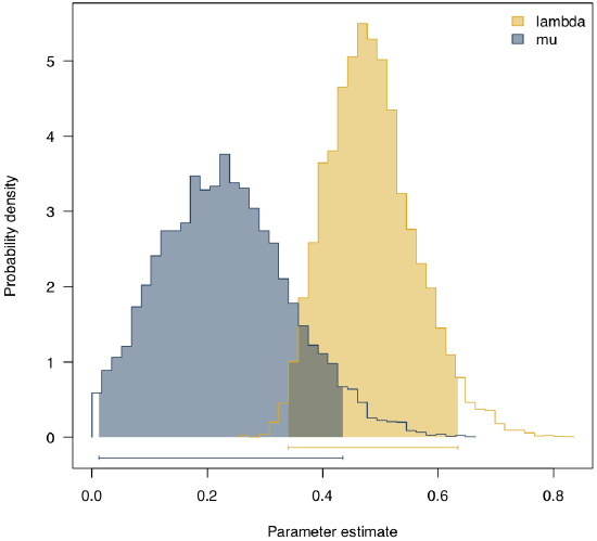
Section 11.4c: Using Bayesian MCMC to fit a Birth-Death Model
We can also estimate birth and death rates using a Bayesian MCMC. We can use exactly the method spelled out above for clade ages and diversities, but substitute Equation \ref{11.11} for the likelihood, thus using the waiting times derived from a phylogenetic tree to estimate model parameters.
Applying this to Lupines with the same priors as before, we obtain the posterior distributions shown in figure 11.5. The mean of the posterior for each parameter is λ = 0.48 and μ = 0.23, quite close to the ML estimates for these parameters.