16.5: Succession

A similar process for more than two species results in a succession of species taking over, one after the other, in an ecological process known as “succession.”

Figure \(\PageIndex{1}\). Multi-species individual growth rate versus resource level, whose time-course is illustrated in Figure \(\PageIndex{2}\)

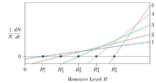
In natural systems many species compete, with tradeoffs between their \(R^{\ast}\) values and their growth rates, as in Figure \(\PageIndex{1}\). The following is a program to simulate the differential equations for five species competing for the same resource and producing the curves of Figure \(\PageIndex{2}\). With only two species, this same program can produce the curves of Figure 16.3.3.

# SIMULATE ONE YEAR 
# This routine simulates competition differential equations through one time
# unit, such as one year, taking very small time steps along the way. 
# Accuracy should be checked by reducing the size of small time steps until 
# the results do not significantly change. 
# This routine implements <Q>Euler’s Method</Q> for solving differential 
# equations, which always works if the time step is small enough. 
#
# ENTRY: ’N1’ to ’N5’ are the starting populations for species 1-5.
#        ’m1’ to ’m5’ specify the sensitivity of the corresponding species
#        to the available amount of resource.
#        ’u1’ to ’u5’ specify the resource tied up in each species. 
#        ’R1star’ to ’R5star’ are the minimum resource levels.
#        ’Rmax’ is the greatest amount of resource possible. 
#        ’dt’ is the duration of each small time step to be taken throughout
#        the year or other time unit.
#
# EXIT:  ’N1’ to ’N5’ are the estimated populations of species 1-5 at the 
#        end of the time unit.
#        ’R’ is the estimated resource level at the end of the time step.

Rmax=R=7;
 R1star=1.0; R2star=2.0; R3star=3.0; R4star=4.0; R5star=5.0;
 N1=0.000001; N2=0.000010; N3=0.000100; N4=0.001000; N5=0.010000;
 m1=0.171468; m2=0.308642; m3=0.555556; m4=1.000000; m5=1.800000; 
 u1=0.001000; u2=0.001000; u3=0.001000; u4=0.001000; u5=0.001000;

# SIMULATE ONE YEAR
SimulateOneYear = function(dt) 
{ for(v in 1:(1/dt))                     # Advance a small time step. 
  { R=Rmax-u1*N1-u2*N2-u3*N3-            # Compute resource remaining.
      u4*N4-u5*N5;
    dN1=m1*(R-R1star)*N1*dt;             # Estimate the change in the 
    dN2=m2*(R-R2star)*N2*dt;             # population of each species. 
    dN3=m3*(R-R3star)*N3*dt; 
    dN4=m4*(R-R4star)*N4*dt; 
    dN5=m5*(R-R5star)*N5*dt;
    
    N1=N1+dN1; N2=N2+dN2;                 # Add the estimated change to 
    N3=N3+dN3; N4=N4+dN4; N5=N5+dN5; }    # each population and repeat.

assign("N1",N1, envir=.GlobalEnv);        # At the end, export the results and return
assign("N2",N2, envir=.GlobalEnv); 
assign("N3",N3, envir=.GlobalEnv); 
assign("N4",N4, envir=.GlobalEnv); 
assign("N5",N5, envir=.GlobalEnv); }

# SIMULATE ALL YEARS
for(t in 0:100)                           # Advance one year. 
{ print(round(c(t,N1,N2,N3,N4,N5)));      # Display results. 
  SimulateOneYear(1/(365*24)); }          # Repeat.

An environment can change because species living in it have effects that can “feed back” and change the environment itself. In this case the feedback is change in the resource level, which each successive species changes in a way that is compatible with its own existence. There is nothing teleological in this; any species that change the environment in ways not compatible with their own existence simply do not persist, and hence are not observed. When the program runs, it produces a file excerpted below, which is graphed in Figure \(\PageIndex{2}\).

t	N1	N2	N3	N4	N5
1	0	0	0	0	0
2	0	0	0	0	13
3	0	0	0	7	391
4	0	0	0	45	1764
5	0	0	1	127	1894
6	0	0	3	329	1743
7	0	0	9	790	1392
:	:	:	:	:	:
60	1649	3536	0	0	0
61	1891	3324	0	0	0
62	2157	3094	0	0	0
63	2445	2864	0	0	0
64	2751	2584	0	0	0
65	3070	2313	0	0	0
66	3397	2039	0	0	0
67	3725	1767	0	0	0
:	:	:	:	:	:
96	5999	1	0	0	0
97	5999	0	0	0	0
98	6000	0	0	0	0
99	6000	0	0	0	0
100	6000	0	0	0	0

Figure \(\PageIndex{2}\). Succession based on the tradeoffs of Figure \(\PageIndex{1}\).

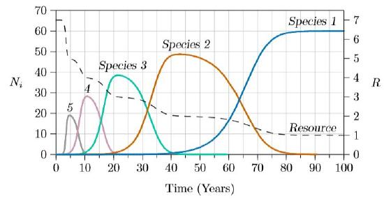
At the beginning in Figure \(\PageIndex{2}\), from time 0 to about time 3, the resource is at its maximum level, \(R_{max}\), and the abundances of all species are at very low levels. Between times 3 and 5—Species 5, the one with the highest growth rate when resources are abundant—increases rapidly while resources drop accordingly. But near the end of that time the next in the series, Species 4, starts to increase, pulling the resource down below the level that allows Species 5 to survive. Species 5 therefore declines while Species 4 increases.

This process continues in succession, with Species 3 replacing 4, 2 replacing 3, and, finally, Species 1 replacing 2. The resource falls in stages as each successive species gains dominance. Finally, when no more superior species exist, the system reaches what is called its “climax condition” at about time 90, with resources at a low level.

There is nothing especially remarkable about Species 1. It is simply (1) the best competitor living in the region, meaning better competitors cannot readily arrive on the scene, or (2) the best competitor that evolutionary processes have yet produced. In either case, it is subject to replacement by another—for example, by an “invasive species” arriving by extraordinary means.

Of course, succession in complex natural systems may not be as clear-cut as in our simple models. Multiple resources are involved, species may be very close to each other in their ecological parameters, and stochastic events may intervene to add confusion.

Figure \(\PageIndex{3}\). Schizacharium at Cedar Creek with oaks invading.