16.3: Resource competition

Competition among two species occurs when the interaction terms \(s_{1,2}\) and \(s_{2,1}\) in Equation 8.1 are both negative. This rather abstract approach does lead to broad insights, but for other kinds of insights let us proceed to a more mechanistic view. Instead of abstract coefficients representing inhibition among species, let us consider resources which species need to thrive and survive. The species will not interact directly— they never even need to come into contact—but will influence each other through their use of a common resource, which they both need for maintenance and growth of their populations.

Resource competition is one of the oldest parts of ecological theory, introduced in the late 1920s by mathematician Vivo Volterra. We will start where he started, considering what have been called “abiotic resources”.

Species require sunlight, space, nitrogen, phosphorous, and other resources in various amounts. If a resource is too rare, populations cannot grow, and in fact will decline. In Figure \(\PageIndex{1}\) this is shown in the region to the left of the arrow marked A, in which the individual growth rate \(1/N\,dN/dt\) is negative.

At higher resource levels the growth rate increases and, at point A, the population can just barely maintain itself. Here the individual growth rate \(1/N\,dN/dt\) is zero. This level of resources is called \(R^{\ast}\), pronounced “are star”. At higher levels of resource, above \(R^{\ast}\), the population grows because \(1/N\,dN/dt\) becomes positive.

Figure \(\PageIndex{1}\) Growth curve generalized for any resource, with a piece-wise linear approximation sketched as dashed lines.

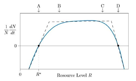
Once resources are abundant—approximately above B in the figure—needs are satiated and the addition of more resources does not make any large difference. Population growth stays approximately the same between marks B and C.

At very high levels, too much resource can actually harm the population. Too much sunlight can burn leaves, for example, while too much nitrogen can damage roots. At this point, above C in Figure \(\PageIndex{1}\), the growth rate starts falling. By D the species can again just barely hold its own, and to the right of D the species is killed by an overabundance of resources.

Figure \(\PageIndex{2}\) Growth curve with only the left linear piece of Figure \(\PageIndex{1}\), usable because species tend to keep resources low.

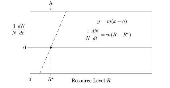
Such high resource levels, however, are not usually observed, because species draw resources concentrations down by using them up. Unless extreme environments are being modeled, only the left dashed linear piece of Figure \(\PageIndex{1}\) needs to be modeled, as shown in Figure \(\PageIndex{2}\).

At this point, it is helpful to review various forms for the equation of a straight line. The usual slope–intercept form, \(y\,=\,mx+b\), which is a y-intercept form—is not as useful here. It’s the x-intercept form, \(y\,=\,m(x−a)\), that comes into play for writing a mechanistic resource model for single species population growth.

1. Slope–intercept form: \(y\,=\,mx\,+\,b\) (slope m, y-intercept b) 2. Intercept–intercept form: \(y\,=\,b(1\,−\,x/a)\) (x-intercept a, y-intercept b) (m = −b/a) 3. Slope–x-intercept form: \(y\,=\,m\,(x − a)\) (slope m, x-intercept a) (b = −m/a)

The zero-growth point, \(R^{\ast}\), is important in the theory of resource competition. It is the amount of resource that just barely sustains the species. If the resource level is less than \(R^{\ast}\), the species dies out; if it is greater, the species grows and expands. The resource level in the environment therefore is expected to be at or near the \(R^{\ast}\) value of the dominant species. If it is above that level, the population grows, new individuals use more resource, and the resource level is consequently reduced until growth stops.

\(R^{\ast}\) can be measured in the greenhouse or the field. In the greenhouse, for example, you might arrange plants in 20 pots and give them different amounts of nitrogen fertilizer in sterile, nutrient-free soil. In the complete absence of fertilizer, the plants will die. With larger amounts of fertilizer the plants will be luxuriant, and when there is too much fertilizer, the resource will become toxic, again leading to dieback in the plants. You can thus measure the curve of Figure \(\PageIndex{1}\) fairly easily and find the point on the left where the plants just survive. This is their \(R^{\ast}\).

You can also measure this value for different species independently, and from the results estimate how plants will fare living together. To start, suppose that one resource is the most limiting. Represent the amount of that limiting resource available in the environment at time \(t\) by the symbol \(R(t)\) or, for shorthand, simply \(R\). The amount in excess of minimal needs is \(R−R^{\ast}\), and that amount of excess will determine the rate of growth. A tiny excess will mean slow growth, but a larger excess can support faster growth. So the equation in Figure \(\PageIndex{2}\) shows the individual growth rate, \(1/N\,dN/dt\), being proportional to how much resource exists in excess.

As before, \(N\) measures the size of the population at time \(t\), in number of individuals, total biomass, or whatever units are relevant to the species being studied. \(R^{\ast}\) is the smallest amount of resource that can support a viable population, and m tells how the individual growth rate, \((1/N)dN/dt\), depends on the amount of resource available in excess of minimal needs.

Now let us say that \(R_{max}\) is the maximum amount of resource available in the environment, in absence of any organisms, and u is the amount of resource used by each living organism in the population. Then \(uN\) is the amount of resource tied up in the population at time \(t\). \(R_{max}\,−\,uN\,=\,R\) is the amount of resource not used by the population. This is the basis of a resource theory that assumes resources are released immediately upon death of an organism, and it has many of the important properties of more complex resource models.

Start with the above statements in algebraic form,

\[\frac{1}{N}\frac{dN}{dt}\,=\,m(R-R^{\ast})\,\,\,and\,\,\,R\,=\,R_{max}\,-uN\]

then substitute the equation on the right above into the one on the left. This gives

\(\frac{1}{N}\frac{dN}{dt}\,=\,m\,(R_{max}\,-\,uN\,-\,R^{\ast})\)

Multiplying through on the right by \(m\) and rearranging terms gives

\[\frac{1}{N}\frac{dN}{dt}\,=\,m(R_{max}\,-\,R^{\ast})\,-\,umN\]

Notice that the first term on the right is a constant and the second term is a constant times N. Does this look familiar? This is just density-regulated population growth in disguise— the \(r\,+\,sN\) model again!

\(\frac{1}{N}\frac{dN}{dt}\,=\,r+sN,\,\,\,r\,=\,m(R_{max}\,-\,R^{/ast}),\,\,\,s\,=\,-um\)

Recall that this also happened for the epidemiological \(I\) model. And it will arise occur again in future models.