10.1: Chapter Introduction
- Page ID
- 25711
This page is a draft and is under active development.

\( \newcommand{\vecs}[1]{\overset { \scriptstyle \rightharpoonup} {\mathbf{#1}} } \)
\( \newcommand{\vecd}[1]{\overset{-\!-\!\rightharpoonup}{\vphantom{a}\smash {#1}}} \)
\( \newcommand{\id}{\mathrm{id}}\) \( \newcommand{\Span}{\mathrm{span}}\)
( \newcommand{\kernel}{\mathrm{null}\,}\) \( \newcommand{\range}{\mathrm{range}\,}\)
\( \newcommand{\RealPart}{\mathrm{Re}}\) \( \newcommand{\ImaginaryPart}{\mathrm{Im}}\)
\( \newcommand{\Argument}{\mathrm{Arg}}\) \( \newcommand{\norm}[1]{\| #1 \|}\)
\( \newcommand{\inner}[2]{\langle #1, #2 \rangle}\)
\( \newcommand{\Span}{\mathrm{span}}\)
\( \newcommand{\id}{\mathrm{id}}\)
\( \newcommand{\Span}{\mathrm{span}}\)
\( \newcommand{\kernel}{\mathrm{null}\,}\)
\( \newcommand{\range}{\mathrm{range}\,}\)
\( \newcommand{\RealPart}{\mathrm{Re}}\)
\( \newcommand{\ImaginaryPart}{\mathrm{Im}}\)
\( \newcommand{\Argument}{\mathrm{Arg}}\)
\( \newcommand{\norm}[1]{\| #1 \|}\)
\( \newcommand{\inner}[2]{\langle #1, #2 \rangle}\)
\( \newcommand{\Span}{\mathrm{span}}\) \( \newcommand{\AA}{\unicode[.8,0]{x212B}}\)
\( \newcommand{\vectorA}[1]{\vec{#1}} % arrow\)
\( \newcommand{\vectorAt}[1]{\vec{\text{#1}}} % arrow\)
\( \newcommand{\vectorB}[1]{\overset { \scriptstyle \rightharpoonup} {\mathbf{#1}} } \)
\( \newcommand{\vectorC}[1]{\textbf{#1}} \)
\( \newcommand{\vectorD}[1]{\overrightarrow{#1}} \)
\( \newcommand{\vectorDt}[1]{\overrightarrow{\text{#1}}} \)
\( \newcommand{\vectE}[1]{\overset{-\!-\!\rightharpoonup}{\vphantom{a}\smash{\mathbf {#1}}}} \)
\( \newcommand{\vecs}[1]{\overset { \scriptstyle \rightharpoonup} {\mathbf{#1}} } \)
\( \newcommand{\vecd}[1]{\overset{-\!-\!\rightharpoonup}{\vphantom{a}\smash {#1}}} \)
\(\newcommand{\avec}{\mathbf a}\) \(\newcommand{\bvec}{\mathbf b}\) \(\newcommand{\cvec}{\mathbf c}\) \(\newcommand{\dvec}{\mathbf d}\) \(\newcommand{\dtil}{\widetilde{\mathbf d}}\) \(\newcommand{\evec}{\mathbf e}\) \(\newcommand{\fvec}{\mathbf f}\) \(\newcommand{\nvec}{\mathbf n}\) \(\newcommand{\pvec}{\mathbf p}\) \(\newcommand{\qvec}{\mathbf q}\) \(\newcommand{\svec}{\mathbf s}\) \(\newcommand{\tvec}{\mathbf t}\) \(\newcommand{\uvec}{\mathbf u}\) \(\newcommand{\vvec}{\mathbf v}\) \(\newcommand{\wvec}{\mathbf w}\) \(\newcommand{\xvec}{\mathbf x}\) \(\newcommand{\yvec}{\mathbf y}\) \(\newcommand{\zvec}{\mathbf z}\) \(\newcommand{\rvec}{\mathbf r}\) \(\newcommand{\mvec}{\mathbf m}\) \(\newcommand{\zerovec}{\mathbf 0}\) \(\newcommand{\onevec}{\mathbf 1}\) \(\newcommand{\real}{\mathbb R}\) \(\newcommand{\twovec}[2]{\left[\begin{array}{r}#1 \\ #2 \end{array}\right]}\) \(\newcommand{\ctwovec}[2]{\left[\begin{array}{c}#1 \\ #2 \end{array}\right]}\) \(\newcommand{\threevec}[3]{\left[\begin{array}{r}#1 \\ #2 \\ #3 \end{array}\right]}\) \(\newcommand{\cthreevec}[3]{\left[\begin{array}{c}#1 \\ #2 \\ #3 \end{array}\right]}\) \(\newcommand{\fourvec}[4]{\left[\begin{array}{r}#1 \\ #2 \\ #3 \\ #4 \end{array}\right]}\) \(\newcommand{\cfourvec}[4]{\left[\begin{array}{c}#1 \\ #2 \\ #3 \\ #4 \end{array}\right]}\) \(\newcommand{\fivevec}[5]{\left[\begin{array}{r}#1 \\ #2 \\ #3 \\ #4 \\ #5 \\ \end{array}\right]}\) \(\newcommand{\cfivevec}[5]{\left[\begin{array}{c}#1 \\ #2 \\ #3 \\ #4 \\ #5 \\ \end{array}\right]}\) \(\newcommand{\mattwo}[4]{\left[\begin{array}{rr}#1 \amp #2 \\ #3 \amp #4 \\ \end{array}\right]}\) \(\newcommand{\laspan}[1]{\text{Span}\{#1\}}\) \(\newcommand{\bcal}{\cal B}\) \(\newcommand{\ccal}{\cal C}\) \(\newcommand{\scal}{\cal S}\) \(\newcommand{\wcal}{\cal W}\) \(\newcommand{\ecal}{\cal E}\) \(\newcommand{\coords}[2]{\left\{#1\right\}_{#2}}\) \(\newcommand{\gray}[1]{\color{gray}{#1}}\) \(\newcommand{\lgray}[1]{\color{lightgray}{#1}}\) \(\newcommand{\rank}{\operatorname{rank}}\) \(\newcommand{\row}{\text{Row}}\) \(\newcommand{\col}{\text{Col}}\) \(\renewcommand{\row}{\text{Row}}\) \(\newcommand{\nul}{\text{Nul}}\) \(\newcommand{\var}{\text{Var}}\) \(\newcommand{\corr}{\text{corr}}\) \(\newcommand{\len}[1]{\left|#1\right|}\) \(\newcommand{\bbar}{\overline{\bvec}}\) \(\newcommand{\bhat}{\widehat{\bvec}}\) \(\newcommand{\bperp}{\bvec^\perp}\) \(\newcommand{\xhat}{\widehat{\xvec}}\) \(\newcommand{\vhat}{\widehat{\vvec}}\) \(\newcommand{\uhat}{\widehat{\uvec}}\) \(\newcommand{\what}{\widehat{\wvec}}\) \(\newcommand{\Sighat}{\widehat{\Sigma}}\) \(\newcommand{\lt}{<}\) \(\newcommand{\gt}{>}\) \(\newcommand{\amp}{&}\) \(\definecolor{fillinmathshade}{gray}{0.9}\)In differential equation models, the basic population dynamics among species become visible at a glance in “phase space.” The concepts and applications of phase spaces were originally worked out late in the ni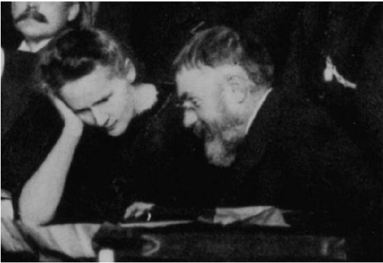 neteenth century by Henri Poincaré and others for the dynamical systems of physics, but the mathematical foundations also apply to the theories of ecology. (At left is Poincaré seated with Marie Curie at the initial Solvay Conference in 1911. As a point of interest, Marie Curie is the only person to have twice won the Nobel Prize for science—and she was nominated the first time before her doctoral defense!)
In a phase space with two species interacting—in competition, predation, or mutualism—the abundance of one species occupies the horizontal axis and that of the other occupies the vertical axis. This makes each possible pair of population values (N1,N2) into a point in the phase space.
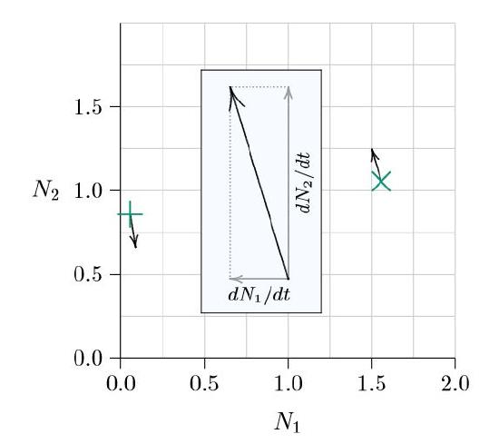
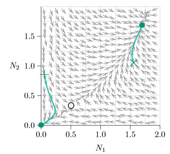
For example, a measured average abundance of 1.55 individuals per square meter for Species 1 and of 1.1 individuals per square meter for Species 2 corresponds to the point marked with an ‘×’ in Figure \(\PageIndex{1}\) — 1.55 units to the right on the horizontal axis and 1.1 units up the vertical axis. If Species 1 is rare, at 0.05 individuals per square meter, and Species 2 is at 0.85 individuals per square meter, the point is that marked with a ‘+’, near the left in Figure \(\PageIndex{1}\). A phase space, however, is not about the size of populations, but rather about how the populations are changing over time. That change \(\frac{dN_1}{dt}\,=\,f_1\,(N_1,\,\,N_2),\frac{dN_2}{dt}\,=\,f_2\,(N_1,\,N_2))\) is made visible as arrows emerging from each point.
Suppose that, at the time of the measurement of the populations marked by ×, Species 1 is decreasing slightly and Species 2 is increasing relatively strongly. Decreasing for Species 1 means moving to the left in the phase space, while increasing for Species 2 means moving up, as shown in the inset of Figure 10.1. The net direction of change would thus be north-northwest. In the opposite direction, for the populations marked by +, if Species 1 is increasing slightly and Species 2 is decreasing relatively strongly, the direction of change would be south-southeast.
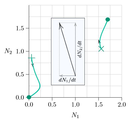
Arrows in the phase space point in the direction of immediate population change. But as the populations change, ecological conditions also change and the paths curve. Figure \(\PageIndex{2}\) shows in green how the populations change in this example as time passes. The pair of abundances starting from × moves up, with Species 1 decreasing at first and then both species increasing and finally coming to rest at the green dot, which marks a joint carrying capacity.
From the +, on the other hand, Species 2 decreases uniformly but Species 1 increases at first and then reverses direction. In this case both species go extinct by arriving at the origin (0,0). Something significant separates the + from the ×.
What separates them can be judged by calculating an arrow at many points throughout the phase space (Figure \(\PageIndex{3}\)). Following the arrows from any pair of abundances (N1,N2) traces the future abundances that will arise as time progresses, and following the arrows backwards shows how the populations could have developed in the past. Note that the arrows seem to be avoiding the open circle near the lower left (at about 0.5, 0.3). That is an Allee point.
Some points in the phase space are exceptional: along certain special curves, the arrows aim exactly horizontally or exactly vertically. This means that one of the two populations is not changing—Species 1 is not changing along the vertical arrows, and Species 2 is unchanged along the horizontal arrows. These special curves are the isoclines—from the roots ‘iso-,’ meaning ‘same’ or ‘equal,’ and ‘-cline,’ meaning ‘slope’ or ‘direction.’)
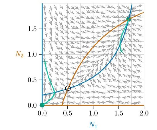
The two isoclines of Species 2 are shown in red in Figure \(\PageIndex{4}\), one along the horizontal axis and the other rising and curving to the right. On the horizontal axis, the abundance of Species 2 is zero. Therefore it will always stay zero, meaning it will not change and making that entire axis an isocline. Along the other red isocline, the arrows emerging exactly from the isocline point exactly right or left, because the system is exactly balanced such that the abundance of Species 2 does not change—it has no vertical movement.
The situation is similar for the two isoclines of Species 1, shown in blue in Figures \(\PageIndex{4}\) and \(\PageIndex{5}\) —one along the vertical axis and the other rising and curving upward. Along the blue curves, the arrows emerging exactly from the isocline point exactly up or down. Again, along the blue isocline the system is exactly balanced such that the abundance of Species 1 does not change—it has no horizontal movement.
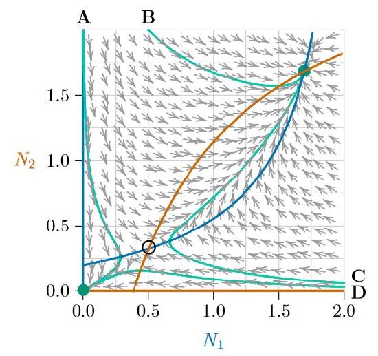
Understanding the isoclines of a system goes a long ways toward understanding the dynamics of the system. Where an isocline of one species meets an isocline of the other, the population of neither species changes and therefore an equilibrium forms. These are marked with circles. Notice that the arrows converge on the filled circles (stable equilibria) and judiciously avoid the open circle (unstable equilibrium). And notice that wherever a population (N1,N2) starts, the arrows carry it to one of two outcomes (except, technically, starting on the Allee point itself, where it would delicately remain until perturbed).
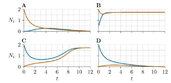
For further illustration, four population growth curves are traced in green in Figure \(\PageIndex{5}\) and marked as A, B, C, and D. All start with one of the populations at 2.0 and the other at a low or moderate level. And they head to one of the two stable equilibria, avoiding the unstable equilibrium in between. You can view these four growth curves plotted in the usual way, as species abundances versus time, in Figure \(\PageIndex{6}\). Blue indicates Species 1, while red indicates Species 2.