17.1: Motif Representation and Information Content
- Page ID
- 41014
\( \newcommand{\vecs}[1]{\overset { \scriptstyle \rightharpoonup} {\mathbf{#1}} } \)
\( \newcommand{\vecd}[1]{\overset{-\!-\!\rightharpoonup}{\vphantom{a}\smash {#1}}} \)
\( \newcommand{\id}{\mathrm{id}}\) \( \newcommand{\Span}{\mathrm{span}}\)
( \newcommand{\kernel}{\mathrm{null}\,}\) \( \newcommand{\range}{\mathrm{range}\,}\)
\( \newcommand{\RealPart}{\mathrm{Re}}\) \( \newcommand{\ImaginaryPart}{\mathrm{Im}}\)
\( \newcommand{\Argument}{\mathrm{Arg}}\) \( \newcommand{\norm}[1]{\| #1 \|}\)
\( \newcommand{\inner}[2]{\langle #1, #2 \rangle}\)
\( \newcommand{\Span}{\mathrm{span}}\)
\( \newcommand{\id}{\mathrm{id}}\)
\( \newcommand{\Span}{\mathrm{span}}\)
\( \newcommand{\kernel}{\mathrm{null}\,}\)
\( \newcommand{\range}{\mathrm{range}\,}\)
\( \newcommand{\RealPart}{\mathrm{Re}}\)
\( \newcommand{\ImaginaryPart}{\mathrm{Im}}\)
\( \newcommand{\Argument}{\mathrm{Arg}}\)
\( \newcommand{\norm}[1]{\| #1 \|}\)
\( \newcommand{\inner}[2]{\langle #1, #2 \rangle}\)
\( \newcommand{\Span}{\mathrm{span}}\) \( \newcommand{\AA}{\unicode[.8,0]{x212B}}\)
\( \newcommand{\vectorA}[1]{\vec{#1}} % arrow\)
\( \newcommand{\vectorAt}[1]{\vec{\text{#1}}} % arrow\)
\( \newcommand{\vectorB}[1]{\overset { \scriptstyle \rightharpoonup} {\mathbf{#1}} } \)
\( \newcommand{\vectorC}[1]{\textbf{#1}} \)
\( \newcommand{\vectorD}[1]{\overrightarrow{#1}} \)
\( \newcommand{\vectorDt}[1]{\overrightarrow{\text{#1}}} \)
\( \newcommand{\vectE}[1]{\overset{-\!-\!\rightharpoonup}{\vphantom{a}\smash{\mathbf {#1}}}} \)
\( \newcommand{\vecs}[1]{\overset { \scriptstyle \rightharpoonup} {\mathbf{#1}} } \)
\( \newcommand{\vecd}[1]{\overset{-\!-\!\rightharpoonup}{\vphantom{a}\smash {#1}}} \)
\(\newcommand{\avec}{\mathbf a}\) \(\newcommand{\bvec}{\mathbf b}\) \(\newcommand{\cvec}{\mathbf c}\) \(\newcommand{\dvec}{\mathbf d}\) \(\newcommand{\dtil}{\widetilde{\mathbf d}}\) \(\newcommand{\evec}{\mathbf e}\) \(\newcommand{\fvec}{\mathbf f}\) \(\newcommand{\nvec}{\mathbf n}\) \(\newcommand{\pvec}{\mathbf p}\) \(\newcommand{\qvec}{\mathbf q}\) \(\newcommand{\svec}{\mathbf s}\) \(\newcommand{\tvec}{\mathbf t}\) \(\newcommand{\uvec}{\mathbf u}\) \(\newcommand{\vvec}{\mathbf v}\) \(\newcommand{\wvec}{\mathbf w}\) \(\newcommand{\xvec}{\mathbf x}\) \(\newcommand{\yvec}{\mathbf y}\) \(\newcommand{\zvec}{\mathbf z}\) \(\newcommand{\rvec}{\mathbf r}\) \(\newcommand{\mvec}{\mathbf m}\) \(\newcommand{\zerovec}{\mathbf 0}\) \(\newcommand{\onevec}{\mathbf 1}\) \(\newcommand{\real}{\mathbb R}\) \(\newcommand{\twovec}[2]{\left[\begin{array}{r}#1 \\ #2 \end{array}\right]}\) \(\newcommand{\ctwovec}[2]{\left[\begin{array}{c}#1 \\ #2 \end{array}\right]}\) \(\newcommand{\threevec}[3]{\left[\begin{array}{r}#1 \\ #2 \\ #3 \end{array}\right]}\) \(\newcommand{\cthreevec}[3]{\left[\begin{array}{c}#1 \\ #2 \\ #3 \end{array}\right]}\) \(\newcommand{\fourvec}[4]{\left[\begin{array}{r}#1 \\ #2 \\ #3 \\ #4 \end{array}\right]}\) \(\newcommand{\cfourvec}[4]{\left[\begin{array}{c}#1 \\ #2 \\ #3 \\ #4 \end{array}\right]}\) \(\newcommand{\fivevec}[5]{\left[\begin{array}{r}#1 \\ #2 \\ #3 \\ #4 \\ #5 \\ \end{array}\right]}\) \(\newcommand{\cfivevec}[5]{\left[\begin{array}{c}#1 \\ #2 \\ #3 \\ #4 \\ #5 \\ \end{array}\right]}\) \(\newcommand{\mattwo}[4]{\left[\begin{array}{rr}#1 \amp #2 \\ #3 \amp #4 \\ \end{array}\right]}\) \(\newcommand{\laspan}[1]{\text{Span}\{#1\}}\) \(\newcommand{\bcal}{\cal B}\) \(\newcommand{\ccal}{\cal C}\) \(\newcommand{\scal}{\cal S}\) \(\newcommand{\wcal}{\cal W}\) \(\newcommand{\ecal}{\cal E}\) \(\newcommand{\coords}[2]{\left\{#1\right\}_{#2}}\) \(\newcommand{\gray}[1]{\color{gray}{#1}}\) \(\newcommand{\lgray}[1]{\color{lightgray}{#1}}\) \(\newcommand{\rank}{\operatorname{rank}}\) \(\newcommand{\row}{\text{Row}}\) \(\newcommand{\col}{\text{Col}}\) \(\renewcommand{\row}{\text{Row}}\) \(\newcommand{\nul}{\text{Nul}}\) \(\newcommand{\var}{\text{Var}}\) \(\newcommand{\corr}{\text{corr}}\) \(\newcommand{\len}[1]{\left|#1\right|}\) \(\newcommand{\bbar}{\overline{\bvec}}\) \(\newcommand{\bhat}{\widehat{\bvec}}\) \(\newcommand{\bperp}{\bvec^\perp}\) \(\newcommand{\xhat}{\widehat{\xvec}}\) \(\newcommand{\vhat}{\widehat{\vvec}}\) \(\newcommand{\uhat}{\widehat{\uvec}}\) \(\newcommand{\what}{\widehat{\wvec}}\) \(\newcommand{\Sighat}{\widehat{\Sigma}}\) \(\newcommand{\lt}{<}\) \(\newcommand{\gt}{>}\) \(\newcommand{\amp}{&}\) \(\definecolor{fillinmathshade}{gray}{0.9}\)Instead of a Profile Matrix, we can also represent Motifs using information theory. In information theory, information about a certain event is communicated through a message. The amount of information carried by a message is measured in bits. We can determine the bits of information carried by a message by observing the probability distribution of the event described in the message. Basically, if we dont know anything about the outcome of the event, the message will contain a lot of bits. However, if we are pretty sure how the event is going to play out, and the message only confirms our suspicions, the message carries very few bits of information. For example, The sentence 0un will rise tomorrow” is not very surprising, so the information of that sentence if quite low.. However, the sentence 0un will not rise tomorrow” is very surprising and it has high information content. We can calculate the specific amount of information in a given message with the equation: − log p.
Shannon Entropy is a measure of the expected amount of information contained in a message. In other words, it is the information contained by a message of every event that could possibly occur weighted by each events probability. The Shannon entropy is given by the equation:
\[ H(X)=-\sum_{i} p_{i} \log _{2} p_{i} \nonumber \]
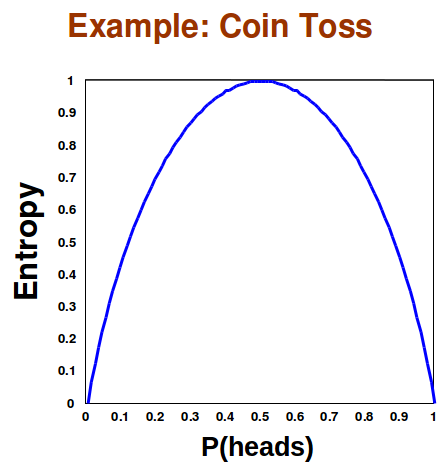
Entropy is maximum when all events have an equal probability of occurring. This is because Entropy tells us the expected amount of information we will learn. If each even has the same chance of occurring we know as little as possible about the event, so the expected amount of information we will learn is maximized. For example, a coin flip has maximal entropy only when the coin is fair. If the coin is not fair, then we know more about the event of the coin flip, and the expected message of the outcome of the coin flip will contain less information.

Figure 17.11: Entropy is maximized when both heads and tails have an equal chance of occurring
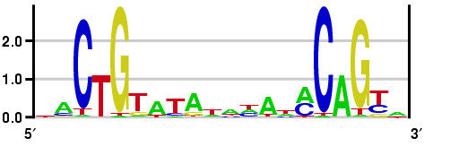
We can model a motif by how much information we have of each position after applying Gibs Sampling or EM. In the following figure, the height of each letter represents the number of bits of information we have learned about that base. Higher stacks correspond to greater certainty about what the base is at that position of the motif while lower stacks correspond to a higher degree of uncertainty. With four codons to choice from, the Shannon Entropy of each position is 2 bits. Another way to look at this figure is that the height of a letter is proportional to the frequency of the base at that position.

Figure 17.12: The height of each stack represents the number of bits of information that Gibbs sampling or EM told us about the postion in the motif
There is a distance metric on probability distributions known as the Kullback-Leibler distance. This allows us to compare the divergence of the motif distribution to some true distribution. The K-L distance is given by
\[ D_{K L}\left(P_{\text {motif}} \mid P_{\text {background}}\right)=\Sigma_{A, T, G, C} P_{\text {motif}}(i) \log \underset{P \text {background}(i)}{P_{\text {motif}}(i)} \nonumber \]
In Plasmodium, there is a lower G-C content. If we assume a G-C content of 20%, then we get the following representation for the above motif. C and G bases are much more unusual, so their prevalence is highly unusual. Note that in this representation, we used the K-L distance, so that it is possible for the stack to be higher than 2.

Figure 17.13: lexA binding site assuming low G-C content and using K-L distance
Bibliography
- [1] Timothy L. Bailey. Fitting a mixture model by expectation maximization to discover motifs in biopoly- mers. In Proceedings of the Second International Conference on Intelligent Systems for Molecular Biology, pages 28–36. AAAI Press, 1994.
- [2] C E Lawrence and A A Reilly. An expectation maximization (em) algorithm for the identification and characterization of common sites in unaligned biopolymer sequences. Proteins, 7(1):41–51, 1990.


