15.3: Clustering Algorithms
- Page ID
- 41003

\( \newcommand{\vecs}[1]{\overset { \scriptstyle \rightharpoonup} {\mathbf{#1}} } \)
\( \newcommand{\vecd}[1]{\overset{-\!-\!\rightharpoonup}{\vphantom{a}\smash {#1}}} \)
\( \newcommand{\id}{\mathrm{id}}\) \( \newcommand{\Span}{\mathrm{span}}\)
( \newcommand{\kernel}{\mathrm{null}\,}\) \( \newcommand{\range}{\mathrm{range}\,}\)
\( \newcommand{\RealPart}{\mathrm{Re}}\) \( \newcommand{\ImaginaryPart}{\mathrm{Im}}\)
\( \newcommand{\Argument}{\mathrm{Arg}}\) \( \newcommand{\norm}[1]{\| #1 \|}\)
\( \newcommand{\inner}[2]{\langle #1, #2 \rangle}\)
\( \newcommand{\Span}{\mathrm{span}}\)
\( \newcommand{\id}{\mathrm{id}}\)
\( \newcommand{\Span}{\mathrm{span}}\)
\( \newcommand{\kernel}{\mathrm{null}\,}\)
\( \newcommand{\range}{\mathrm{range}\,}\)
\( \newcommand{\RealPart}{\mathrm{Re}}\)
\( \newcommand{\ImaginaryPart}{\mathrm{Im}}\)
\( \newcommand{\Argument}{\mathrm{Arg}}\)
\( \newcommand{\norm}[1]{\| #1 \|}\)
\( \newcommand{\inner}[2]{\langle #1, #2 \rangle}\)
\( \newcommand{\Span}{\mathrm{span}}\) \( \newcommand{\AA}{\unicode[.8,0]{x212B}}\)
\( \newcommand{\vectorA}[1]{\vec{#1}} % arrow\)
\( \newcommand{\vectorAt}[1]{\vec{\text{#1}}} % arrow\)
\( \newcommand{\vectorB}[1]{\overset { \scriptstyle \rightharpoonup} {\mathbf{#1}} } \)
\( \newcommand{\vectorC}[1]{\textbf{#1}} \)
\( \newcommand{\vectorD}[1]{\overrightarrow{#1}} \)
\( \newcommand{\vectorDt}[1]{\overrightarrow{\text{#1}}} \)
\( \newcommand{\vectE}[1]{\overset{-\!-\!\rightharpoonup}{\vphantom{a}\smash{\mathbf {#1}}}} \)
\( \newcommand{\vecs}[1]{\overset { \scriptstyle \rightharpoonup} {\mathbf{#1}} } \)
\( \newcommand{\vecd}[1]{\overset{-\!-\!\rightharpoonup}{\vphantom{a}\smash {#1}}} \)
\(\newcommand{\avec}{\mathbf a}\) \(\newcommand{\bvec}{\mathbf b}\) \(\newcommand{\cvec}{\mathbf c}\) \(\newcommand{\dvec}{\mathbf d}\) \(\newcommand{\dtil}{\widetilde{\mathbf d}}\) \(\newcommand{\evec}{\mathbf e}\) \(\newcommand{\fvec}{\mathbf f}\) \(\newcommand{\nvec}{\mathbf n}\) \(\newcommand{\pvec}{\mathbf p}\) \(\newcommand{\qvec}{\mathbf q}\) \(\newcommand{\svec}{\mathbf s}\) \(\newcommand{\tvec}{\mathbf t}\) \(\newcommand{\uvec}{\mathbf u}\) \(\newcommand{\vvec}{\mathbf v}\) \(\newcommand{\wvec}{\mathbf w}\) \(\newcommand{\xvec}{\mathbf x}\) \(\newcommand{\yvec}{\mathbf y}\) \(\newcommand{\zvec}{\mathbf z}\) \(\newcommand{\rvec}{\mathbf r}\) \(\newcommand{\mvec}{\mathbf m}\) \(\newcommand{\zerovec}{\mathbf 0}\) \(\newcommand{\onevec}{\mathbf 1}\) \(\newcommand{\real}{\mathbb R}\) \(\newcommand{\twovec}[2]{\left[\begin{array}{r}#1 \\ #2 \end{array}\right]}\) \(\newcommand{\ctwovec}[2]{\left[\begin{array}{c}#1 \\ #2 \end{array}\right]}\) \(\newcommand{\threevec}[3]{\left[\begin{array}{r}#1 \\ #2 \\ #3 \end{array}\right]}\) \(\newcommand{\cthreevec}[3]{\left[\begin{array}{c}#1 \\ #2 \\ #3 \end{array}\right]}\) \(\newcommand{\fourvec}[4]{\left[\begin{array}{r}#1 \\ #2 \\ #3 \\ #4 \end{array}\right]}\) \(\newcommand{\cfourvec}[4]{\left[\begin{array}{c}#1 \\ #2 \\ #3 \\ #4 \end{array}\right]}\) \(\newcommand{\fivevec}[5]{\left[\begin{array}{r}#1 \\ #2 \\ #3 \\ #4 \\ #5 \\ \end{array}\right]}\) \(\newcommand{\cfivevec}[5]{\left[\begin{array}{c}#1 \\ #2 \\ #3 \\ #4 \\ #5 \\ \end{array}\right]}\) \(\newcommand{\mattwo}[4]{\left[\begin{array}{rr}#1 \amp #2 \\ #3 \amp #4 \\ \end{array}\right]}\) \(\newcommand{\laspan}[1]{\text{Span}\{#1\}}\) \(\newcommand{\bcal}{\cal B}\) \(\newcommand{\ccal}{\cal C}\) \(\newcommand{\scal}{\cal S}\) \(\newcommand{\wcal}{\cal W}\) \(\newcommand{\ecal}{\cal E}\) \(\newcommand{\coords}[2]{\left\{#1\right\}_{#2}}\) \(\newcommand{\gray}[1]{\color{gray}{#1}}\) \(\newcommand{\lgray}[1]{\color{lightgray}{#1}}\) \(\newcommand{\rank}{\operatorname{rank}}\) \(\newcommand{\row}{\text{Row}}\) \(\newcommand{\col}{\text{Col}}\) \(\renewcommand{\row}{\text{Row}}\) \(\newcommand{\nul}{\text{Nul}}\) \(\newcommand{\var}{\text{Var}}\) \(\newcommand{\corr}{\text{corr}}\) \(\newcommand{\len}[1]{\left|#1\right|}\) \(\newcommand{\bbar}{\overline{\bvec}}\) \(\newcommand{\bhat}{\widehat{\bvec}}\) \(\newcommand{\bperp}{\bvec^\perp}\) \(\newcommand{\xhat}{\widehat{\xvec}}\) \(\newcommand{\vhat}{\widehat{\vvec}}\) \(\newcommand{\uhat}{\widehat{\uvec}}\) \(\newcommand{\what}{\widehat{\wvec}}\) \(\newcommand{\Sighat}{\widehat{\Sigma}}\) \(\newcommand{\lt}{<}\) \(\newcommand{\gt}{>}\) \(\newcommand{\amp}{&}\) \(\definecolor{fillinmathshade}{gray}{0.9}\)To analyze the gene expression data, it is common to perform clustering analysis. There are two types of clustering algorithms: partitioning and agglomerative. Partitional clustering divides objects into non- overlapping clusters so that each data object is in one subset. Alternatively, agglomerative clustering methods yield a set of nested clusters organized as a hierarchy representing structures from broader to finer levels of detail.
K-Means Clustering
The k-means algorithm clusters n objects based on their attributes into k partitions. This is an example of partitioning, where each point is assigned to exactly one cluster such that the sum of distances from each point to its correspondingly labeled center is minimized. The motivation underlying this process is to make the most compact clusters possible, usually in terms of a Euclidean distance metric.
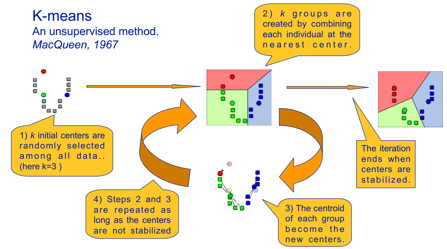
The k-means algorithm, as illustrated in figure 15.8, is implemented as follows:
- Assume a fixed number of clusters, k
- Initialization: Randomly initialize the k means μk associated with the clusters and assign each data point xi to the nearest cluster, where the distance between xi and μk is given by di,k = (xi − μk)2 .
- Iteration: Recalculate the centroid of the cluster given the points assigned to it: \(\mu_{k}(n+1)=\sum_{x_{i} \in k} \frac{x_{i}}{\left|x^{k}\right|}\) where xk is the number of points with label k. Reassign data points to the k new centroids by the given distance metric. The new centers are effectively calculated to be the average of the points assigned to each cluster.
- Termination: Iterate until convergence or until a user-specified number of iterations has been reached. Note that the iteration may be trapped at some local optima.
There are several methods for choosing k: simply looking at the data to identify potential clusters or iteratively trying values for n, while penalizing model complexity. We can always make better clusters by increasing k, but at some point we begin overfitting the data.
We can also think of k-means as trying to minimize a cost criterion associated with the size of each cluster, where the cost increases as the clusters get less compact. However, some points can be almost halfway between two centers, which doesn’t fit well with the binary belonging k-means clustering.
Fuzzy K-Means Clustering
In fuzzy clustering, each point has a probability of belonging to each cluster, rather than completely belonging to just one cluster. Fuzzy k-means specifically tries to deal with the problem where points are somewhat in between centers or otherwise ambiguous by replacing distance with probability, which of course could be some function of distance, such as having probability relative to the inverse of the distance. Fuzzy k-means uses a weighted centroid based on those probabilities. Processes of initialization, iteration, and termination are the same as the ones used in k-means. The resulting clusters are best analyzed as probabilistic distributions rather than a hard assignment of labels. One should realize that k-means is a special case of fuzzy k-means when the probability function used is simply 1 if the data point is closest to a centroid and 0 otherwise.
The fuzzy k-means algorithm is the following:
- Assume a fixed number of clusters k
- Initialization: Randomly initialize the k means μk associated with the clusters and compute the probability that each data point xi is a member of a given cluster k, P(point xi has label k|xi,k).
- Iteration: Recalculate the centroid of the cluster as the weighted centroid given the probabilities of membership of all data points xi: \[\mu_{k}(n+1)=\frac{\sum_{x_{i} \in k} x_{i} \times P\left(\mu_{k} \mid x_{i}\right)^{b}}{\sum_{x_{i} \in k} P\left(\mu_{k} \mid x_{i}\right)^{b}} \nonumber \] And recalculate updated memberships P (μk|xi)(there are different ways to define membership, here is just one example): \[P\left(\mu_{k} \mid x_{i}\right)=\left(\sum_{j=1}^{k}\left(\frac{d_{i k}}{d_{j k}}\right)^{\frac{2}{b-1}}\right)^{-1} \nonumber \]
- Termination: Iterate until membership matrix converges or until a user-specified number of iterations has been reached (the iteration may be trapped at some local maxima or minima)
The b here is the weighting exponent which controls the relative weights places on each partition, or the degree of fuzziness. When b− > 1, the partitions that minimize the squared error function is increasingly hard (non-fuzzy), while as b− > ∞ the memberships all approach 1 , which is the fuzziest state. There is no k theoretical evidence of how to choose an optimal b, while the empirical useful values are among [1, 30], and in most of the studies, 1.5 \(\leqslant \) b \(\legslant \) 3.0 worked well.
K-Means as a Generative Model
A generative model is a model for randomly generating observable-data values, given some hidden parameters. While a generative model is a probability model of all variables, a discriminative model provides a conditional model only of the target variable(s) using the observed variables.
In order to make k-means a generative model, we now look at it in a probabilistic manner, where we assume that data points in cluster k are generated using a Gaussian distribution with the mean on the center of cluster and a variance of 1, which gives
\[P\left(x_{i} \mid \mu_{k}\right)=\frac{1}{\sqrt{2 \pi}} \exp \left\{-\frac{\left(x_{i}-\mu_{k}\right)^{2}}{2}\right\}.\]
This gives a stochastic representation of the data, as shown in figure 15.10. Now this turns to a maximum likelihood problem, which, we will show in below, is exactly equivalent to the original k-means algorithm mentioned above.
.png?revision=1&size=bestfit&width=1001&height=334)
In the generating step, we want to find a most likely partition, or assignment of label, for each xi given the mean μk. With the assumption that each point is drawn independently, we could look for the maximum likelihood label for each point separately:
\[\arg \max _{k} P\left(x_{i} \mid \mu_{k}\right)=\arg \max _{k} \frac{1}{\sqrt{2 \pi}} \exp \left\{-\frac{\left(x_{i}-\mu_{k}\right)^{2}}{2}\right\}=\arg \min _{k}\left(x_{i}-\mu_{k}\right)^{2} \nonumber \]
This is totally equivalent to finding the nearest cluster center in the original k-means algorithm.
In the Estimation step, we look for the maximum likelihood estimate of the cluster mean μk, given the partitions (labels):
\[ \left.\arg \max _{\mu}\left\{\log \prod_{i} P\left(x_{i} \mid \mu\right)\right\}=\arg \max _{\mu} \sum_{i}\left\{-\frac{1}{2}\left(x_{i}-\mu\right)^{2}+\log \left(\frac{1}{\sqrt{2 \pi}}\right)\right)\right\}=\arg \min _{\mu} \sum_{i}\left(x_{i}-\mu\right)^{2} \nonumber \]
Note that the solution of this problem is exactly the centroid of the xi, which is the same procedure as the original k-means algorithm.
Unfortunately, since k-means assumes independence between the axes, covariance and variance are not accounted for using k-means, so models such as oblong distributions are not possible. However, this issue can be resolved when generalize this problem into expectation maximization problem.
Expectation Maximization
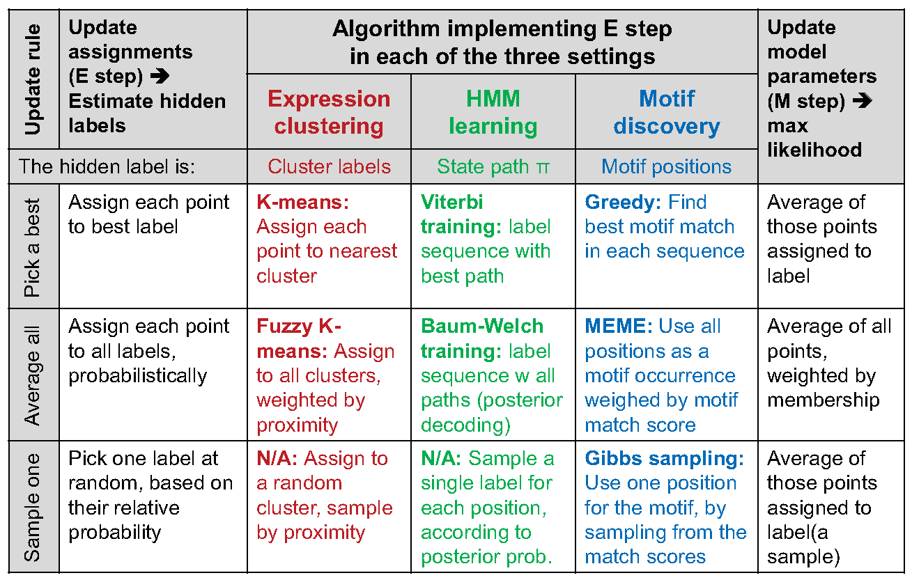
K-means can be seen as an example of EM (expectation maximization algorithms), as shown in figure 15.11 where expectation consists of estimation of hidden labels, Q, and maximizing of expected likelihood occurs given data and Q. Assigning each point the label of the nearest center corresponds to the E step of estimating the most likely label given the previous parameter. Then, using the data produced in the E step as observation, moving the centroid to the average of the labels assigned to that center corresponds to the M step of maximizing the likelihood of the center given the labels. This case is analogous to Viterbi learning. A similar comparison can be drawn for fuzzy k-means, which is analogous to Baum-Welch from HMMs. Figure 15.12 compares clustering, HMM and motif discovery with respect to expectation minimization algorithm.
It should be noted that using the EM framework, the k means approach can be generalized to clusters of oblong shape and varying sizes. With k means, data points are always assigned to the nearest cluster center. By introducing a covariance matrix to the Gaussian probability function, we can allow for clusters of different sizes. By setting the variance to be different along different axes, we can even create oblong distributions.
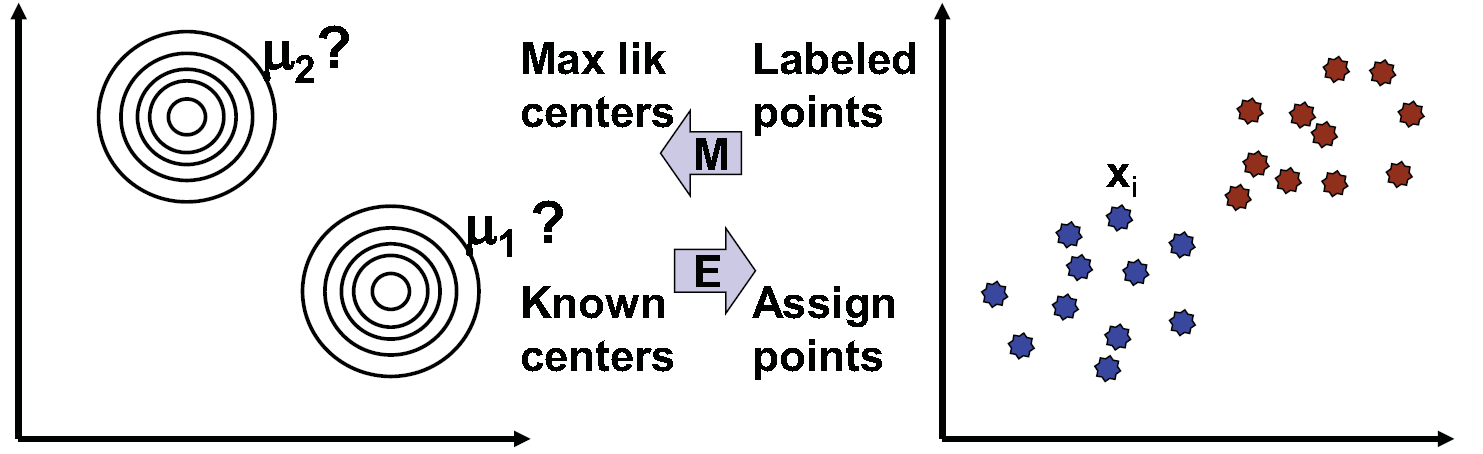
Figure 15.11: K-Means as an expectation maximization (EM) algorithm.
EM is guaranteed to converge and guaranteed to find the best possible answer, at least from an algorithmic point of view. The notable problem with this solution is that the existence of local maxima of probability density can prevent the algorithm from convergin to the global maximum. One approach that may avoid this complication is to attempt multiple initializations to better determine the landscape of probabilities.
The limitations of the K-Means algorithm
The k-means algorithm has a few limitations which are important to keep in mind when using it and before choosing it. First of all, it requires a metric. For example, we cannot use the k-means algorithm on a set of words since we would not have any metric.
The second main limitation of the k-means algorithm is its sensitivity to noise. One way to try to reduce the noise is to run a principle component analysis beforehand. Another way is to weight each variable in order to give less weight to the variables affected by significant noise: the weights will be calculated dynamically at each iteration of the algorithm K-means [3].
The third limitation is that the choice of initial centers can influence the results. There exist heuristics to select the initial cluster centers, but none of them are perfect.
Lastly, we need to know a priori the number of classes. As we have seen, there are ways to circumvent this problem, essentially by running several times the algorithm while varying k or using the rule of thumb \(k \approx \sqrt{n / 2} if we are short on the computational side. en.Wikipedia.org/wiki/Determining_ the_number_of_clusters_in_a_data_set summarizes well the different techniques to select the number of clusters. Hierarchical clustering provides a handy approach to choosing the number of cluster.
Hierarchical Clustering
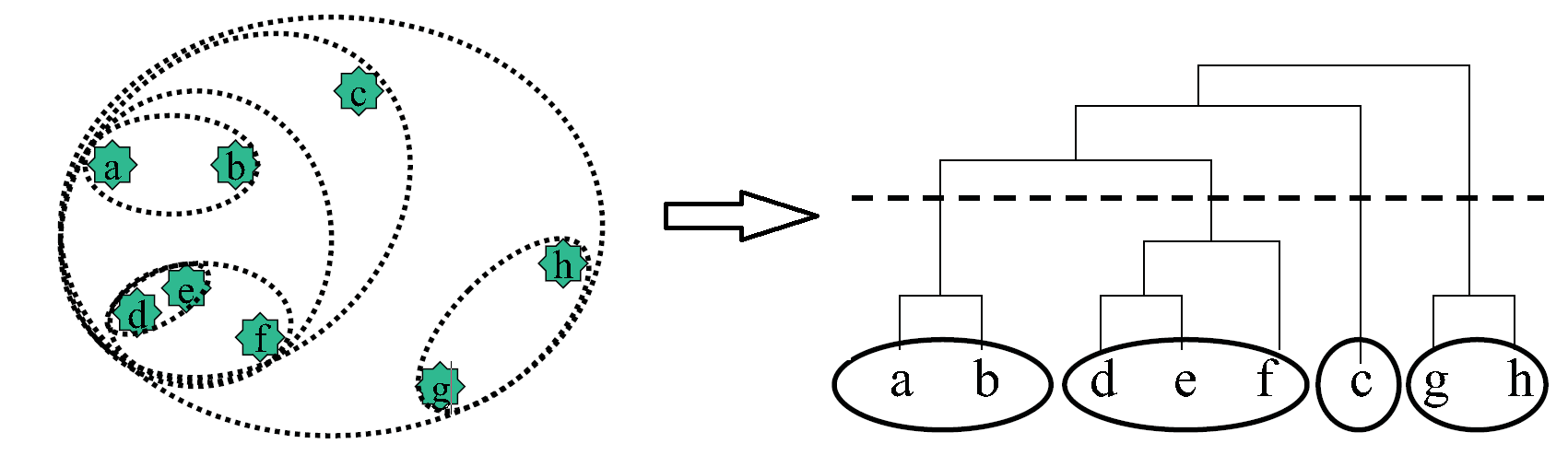
While the clustering discussed thus far often provide valuable insight into the nature of various data, they generally overlook an essential component of biological data, namely the idea that similarity might exist on multiple levels. To be more precise, similarity is an intrinsically hierarchical property, and this aspect is not addressed in the clustering algorithms discussed thus far. Hierarchical clustering specifically addresses this in a very simple manner, and is perhaps the most widely used algorithm for expression data. As illustrated in figure 15.13, it is implemented as follows:
1. Initialization: Initialize a list containing each point as an independent cluster.
2. Iteration: Create a new cluster containing the two closest clusters in the list. Add this new cluster to
the list and remove the two constituent clusters from the list.
One key benefit of using hierarchical clustering and keeping track of the times at which we merge certain clusters is that we can create a tree structure that details the times at which we joined every cluster, as can be seen in figure 15.13. Thus, to get a number of clusters that fits your problem, you simply cut at a cut-level of your choice as in figure 15.13 and that gives you the number of clusters corresponding to that cut-level. However, be aware that one potential pitfall with this approach is that at certain cut-levels, elements that are fairly close in space (such as e and b in figure 15.13), might not be in the same cluster.
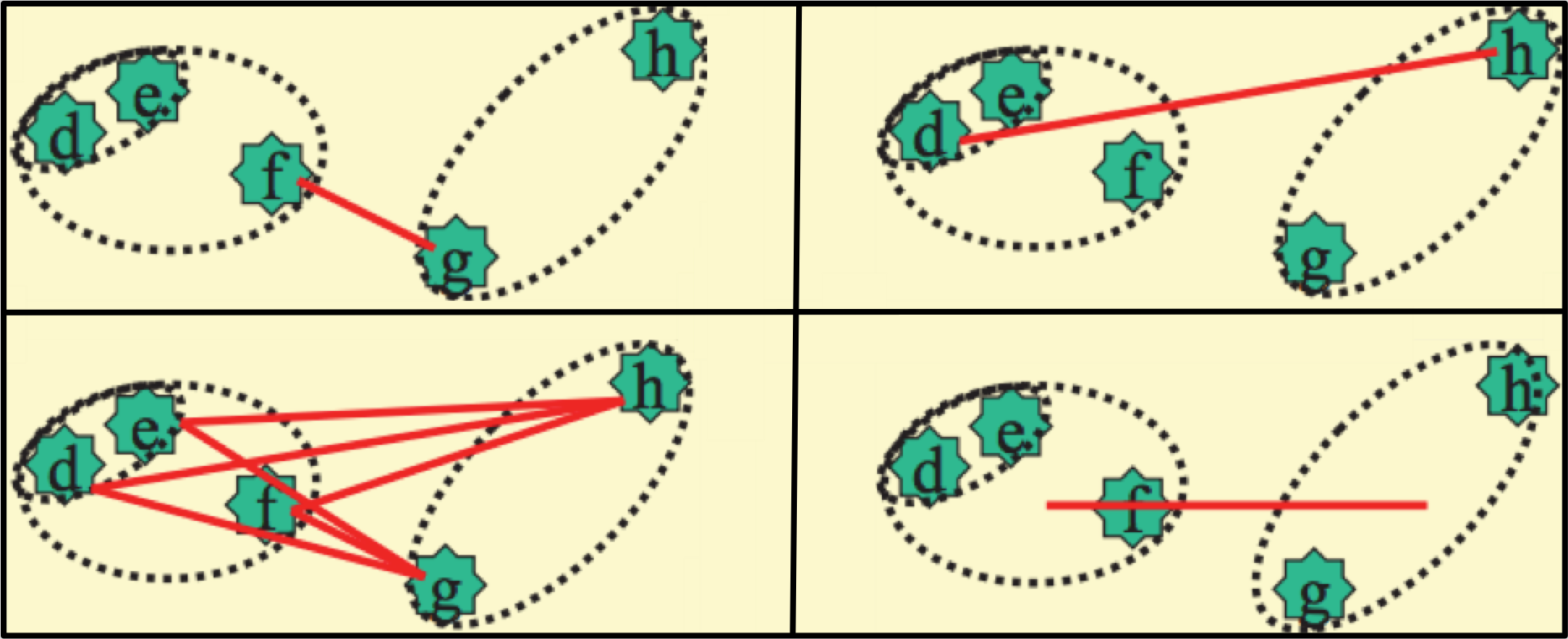
Of course, a method for determining distances between clusters is required. The particular metric used varies with context, but (as can be seen in figure 15.14 some common implementations include the maximum,
minimum, and average distances between constituent clusters, and the distance between the centroids of the clusters.
Noted that when choosing the closest clusters, calculating all pair-wise distances is very time and space consuming, therefore a better scheme is needed. One possible way of doing this is : 1) define some bounding boxes that divide the feature space into several subspaces 2) calculate pair-wise distances within each box 3)shift the boundary of the boxes in different directions and recalculate pair-wise distances 4) choose the closest pair based on the results in all iterations.
Evaluating Cluster Performance
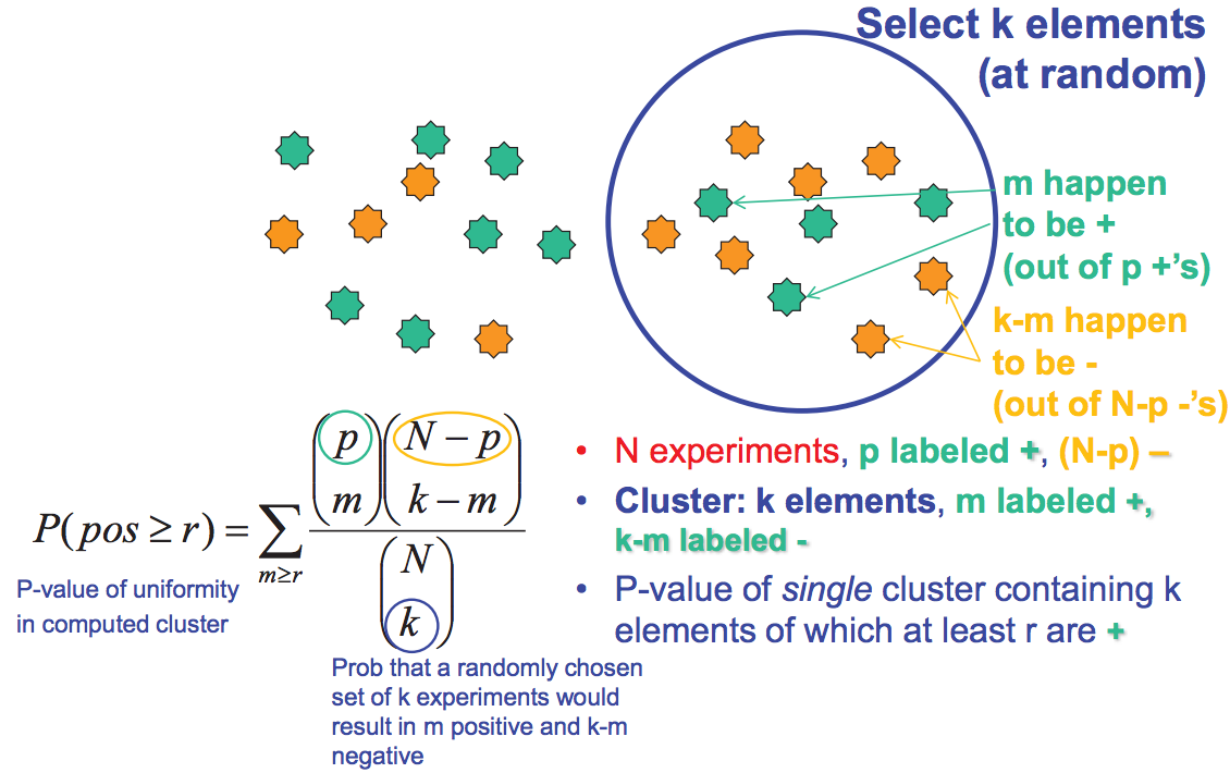
The validity of a particular clustering can be evaluated in a number of different ways. The overrepresentation of a known group of genes in a cluster, or, more generally, correlation between the clustering and confirmed biological associations, is a good indicator of validity and significance. If biological data is not yet available, however, there are ways to assess validity using statistics. For instance, robust clusters will appear from clustering even when only subsets of the total available data are used to generate clusters. In addition, the statistical significance of a clustering can be determined by calculating the probability of a particular distribution having been obtained randomly for each cluster. This calculation utilizes variations on the hypergeometric distribution. As can be seen from figure 15.15, we can do this by calculating the probability that we have more than r +’s when we pick k elements from a total of N elements. http://en.Wikipedia.org/wiki/Cluster...tering_results gives several formula to assess the quality of the clustering.