
15.2: Methods for Measuring Gene Expression
- Page ID
- 41002

The most intuitive way to investigate a certain phenotype is to measure the expression levels of functional proteins present at a given time in the cell. However, measuring the concentration of proteins can be difficult, due to their varying locations, modifications, and contexts in which they are found, as well as due to the incompleteness of the proteome. mRNA expression levels, however, are easier to measure, and are often a good approximation. By measuring the mRNA, we analyze regulation at the transcription level, without the added complications of translational regulation and active protein degradation, which simplifies the analysis at the cost of losing information. In this chapter, we will consider two techniques for generating gene expression data: microarrays and RNA-seq.
Microarrays
Microarrays allow the analysis of the expression levels of thousands of preselected genes in one experiment. The basic principle behind microarrays is the hybridization of complementary DNA fragments. To begin, short segments of DNA, known as probes, are attached to a solid surface, commonly known as a gene chip. Then, the RNA population of interest, which has been taken from a cell, is reverse transcribed to cDNA (complementary DNA) via reverse transcriptase, which synthesizes DNA from RNA using the poly-A tail as a primer. For intergenic sequences which have no poly-A tail, a standard primer can be ligated to the ends of the mRNA. The resulting DNA has more complementarity to the DNA on the slide than the RNA. The cDNA is than washed over the chip and the resulting hybridization triggers the probes to fluoresce. This can be detected to determine the relative abundance of the mRNA in the target, as illustrated in figure 15.2.

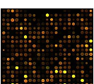
Figure 15.2: Gene expression values from microarray experiments can be represented as heat maps to visualize the result of data analysis.
Two basic types of microarrays are currently used. Affymetrix gene chips have one spot for every gene and have longer probes on the order of 100s of nucleotides. On the other hand, spotted oligonucleotide arrays tile genes and have shorter probes around the tens of bases.
There are numerous sources of error in the current methods and future methods seek to remove steps in the process. For instance, reverse transcriptase may introduce mismatches, which weaken interaction with the correct probe or cause cross hybridization, or binding to multiple probes. One solution to this has been to use multiple probes per gene, as cross hybridization will be different for each gene. Still, reverse transcription is necessary due to the secondary structure of RNA. The structural stability of DNA makes it less probable to bend and not hybridize to the probe. The next generation of technologies, such as RNA-Seq, sequences the RNA as it comes out of the cell, essentially probing every base of the genome.
RNA-seq
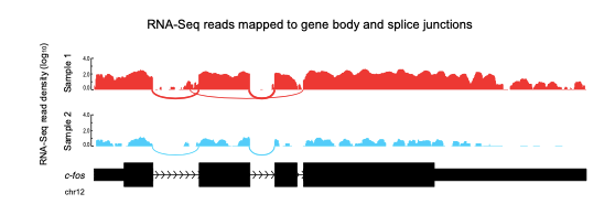
Figure 15.3: RNA-Seq reads mapping to a gene (c-fos) and its splice junctions. Densities along exon represent read densities mapping to exons (in log10), arcs correspond to junction reads, where arc width is drawn in proportion to number of reads in that junction. The gene is downregulated in Sample 2 compared to Sample 1.
RNA-Seq, also known as whole transcriptome shotgun sequencing, attempts to perform the same function that DNA microarrays have been used to perform in the past, but with greater resolution. In particular, DNA microarrays utilize specific probes, and creation of these probes necessarily depends on prior knowledge of the genome and the size of the array being produced. RNA-seq removes these limitations by simply sequencing all of the cDNA produced in microarray experiments. This is made possible by next-generation sequencing technology. The technique has been rapidly adopted in studies of diseases like cancer [4]. The data from RNA-seq is then analyzed by clustering in the same manner as data from microarrays would normally be analyzed.
Gene Expression Matrices
Microarrays and RNA-seq are frequently used to compare the gene expression profiles of cells under various conditions. The amount of data generated from these experiments is enormous. Microarrays can analyze thousands of genes, and RNA-seq can, in principle, analyze every gene that is actively expressed. The expression level of each of those genes is measured across a variety of conditions, including time courses, stages of development, phenotypes, healthy vs. sick, and other factors.
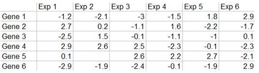
To understand what the heatmap of a gene expression matrix (Figure 15.4) convey, we have to first understand what the expression data matrix tells us. By using microarrays and RNA-seq, we can obtain gene expression level in quantitative form in an experiment. If we have multiple experiments, we can construct a value matrix (Figure 15.5) representing a log value of (T/R), where T is the gene expression level in test sample and R is the gene expression level in reference sample.
The Expression Matrix removed due to copyright restrictions.
Figure 15.4: Transforming Figure 4 to a heatmap
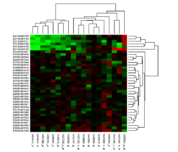
If we visualize the matrix as a heatmap, then we obtain the following new colored-matrix:
These matrices can be clustered hierarchically showing the relation between pairs of genes, pairs of pairs, and so on, creating a dendrogram in which the rows and columns can be ordered using optimal leaf ordering algorithms.
Image in the public domain. This graph was generated using the program Cluster from Michael Eisen, which is available from rana.lbl.gov/EisenSoftware.htm, with data extracted from the StemBase database of gene expression data.
By revealing the hidden structure of a long segment of genome, we obtain great insight of what a fragment of gene does, and subsequently understand more about the root cause of an unknown disease.
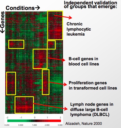
Source: Alizadeh, Ash A., Michael B. Eisen, et al. "Distinct Types of Diffuse Large B-cell Lymphoma Identified by Gene Expression Profiling." Nature 403, no. 6769 (2000): 503-11.
Figure 15.7: Using gene expression matrix to infer more about a disease and gene segment
This predictive and analytical power is increased due to the ability of biclustering the data; that is, clustering along both dimensions of the matrix. The matrix allows for the comparison of expression profiles of genes, as well as comparing the similarity of different conditions such as diseases. A challenge, though, is the curse of dimensionality. As the space of the data increases, the clustering of the points diminishes. Sometimes, the data can be reduced to lower dimensional spaces to find structure in the data using clustering to infer which points belong together based on proximity.
Interpreting the data can also be a challenge, since there may be other biological phenomena in play. For example, protein-coding exons have higher intensity, due to the fact that introns are rapidly degraded. At the same time, not all introns are junk and there may be ambiguities in alternative splicing. There are also cellular mechanisms that degrade aberrant transcripts through non-sense mediated decay.