
15.1: Introduction
- Page ID
- 41001

In this chapter, we consider the problem of discerning similarities or patterns within large datasets. Finding structure in such data sets allows us to draw conclusions about the process as well as the structure underlying the observations. We approach this problem through the application of clustering techniques. The following chapter will focus on classification techniques.
Clustering vs Classification
One important distinction to be made early on is the difference between classification and clustering. Clas- sification is the problem of identifying to which of a set of categories (sub-populations) a new observation belongs, on the basis of a training set of data containing observations or instances whose category member- ship is known. The training set is used to learn rules that will accurately assign labels to new observations. The difficulty is to find the most important features (feature selection).
In the terminology of machine learning, classification is considered an instance of supervised learning, i.e. learning where a training set of correctly-identified observations is available. The corresponding unsupervised procedure is known as clustering or cluster analysis, and involves grouping data into categories based on some measure of inherent similarity, such as the distance between instances, considered as vectors in a multi- dimensional vector space. The difficulty is to identify the structure of the data. Figure 15.1 illustrates the difference between clustering and classification.
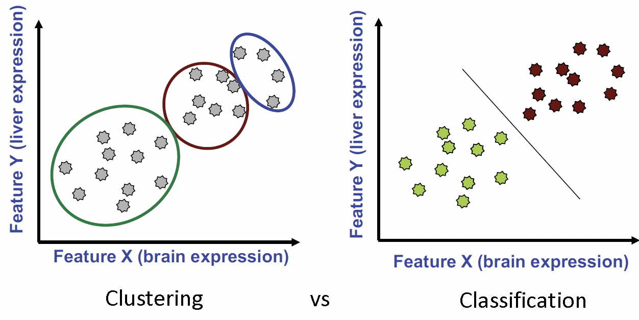
Figure 15.1: Clustering compared to classification. In clustering we group observations into clusters based on how near they are to one another. In classification we want a rule that will accurately assign labels to new points.
Applications
Clustering was originally developed within the field of artificial intelligence. Being able to group similar objects, with full implications of generality implied, is indeed a fairly desirable attribute for an artificial intelligence, and one that humans perform routinely throughout life. As the development of clustering algorithms proceeded apace, it quickly becomes clear that there was no intrinsic barrier involved in applying these algorithms to larger and larger datasets. This realization led to the rapid introduction of clustering to computational biology and other fields dealing with large datasets.
Clustering has many applications to computational biology. For example, let’s consider expression profiles of many genes taken at various developmental stages. Clustering may show that certain sets of genes line up (i.e. show the same expression levels) at various stages. This may indicate that this set of genes has common expression or regulation and we can use this to infer similar function. Furthermore, if we find a uncharacterized gene in such a set of genes, we can reason that the uncharacterized gene also has a similar function through guilt by association.
Chromatin marks and regulatory motifs can be used to predict logical relationships between regulators and target genes in a similar manner. This sort of analysis enables the construction of models that allow us to predict gene expression. These models can be used to modify the regulatory properties of a particular gene, predict how a disease state arose, or aid in targeting genes to particular organs based on regulatory circuits in the cells of the relevant organ.
Computational biology deals with increasingly large and open-access datasets. One such example is the ENCODE project [2]. Launched is 2003, the goal of ENCODE is to build a comprehensive list of functional elements in the human genome, including elements that act at the protein and RNA levels, and regulatory elements that control cells and circumstances in which a gene is active. ENCODE data are now freely and immediately available for the entire human genome: http://genome.ucsc.edu/ENCODE/. Using all of this data, it is possible to make functional predictions about genes through the use of clustering.