
12.4: Practical topic- RNAseq
- Page ID
- 40988

RNA-seq is a method that utilizes next-generation sequencing technology to sequence cDNA allowing us to gain insight into the contents of RNA. The two main problems that RNA-seq addresses are (1) discover new genes such as splice isoforms of previously discovered genes and (2) uncover the expression levels of genes and transcripts from the sequencing data. Additionally, RNA-seq is also beginning to replace many traditional sequencing techniques allowing labs to perform experiments more efficiently.
How it works
The RNA-Seq machine grabs a transcript and breaks it into different fragments, where the fragments are normally distributed. With the speed that the RNA-seq can sequence these transcript fragments (or reads), there are an abundant number of reads allowing us to extract expression levels. The basic idea behind this method relies on the fact that the more abundant a transcript is, the more fragments we’ll sequence from it.
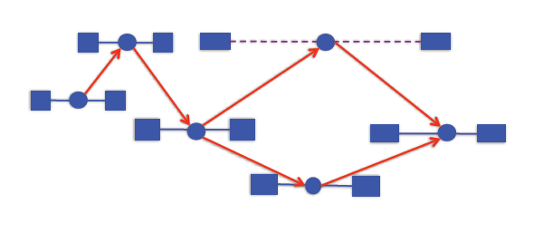
The tools used to analyze RNA-Seq data are collectively known as the “Tuxedo Tools”
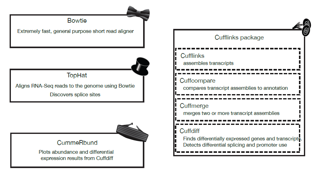
Figure 12.1: Tuxedo Tools
Aligning RNA-Seq reads to genomes and transcriptomes
Since RNA-Seq produces so many reads, the alignment algorithm must have a fast runtime, approximately of the order of O(n). There are two main strategies for aligning short reads, which require that we already have the transcripts.
1. Spaced seeds indexing
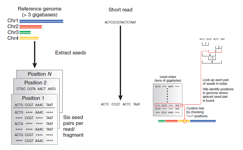
Figure 12.2: How spaced seeds indexing works
Spaced seeds indexing involves taking each read and breaking it into fragments, or “seeds”. We take every combination of two fragments (“seed pairs”) and compare them to an index of seeds (which will take tens of gigabytes of space) for potential hits. Compare the other seeds to the index to make sure we have a hit.
2. Burrows-Wheeler indexing
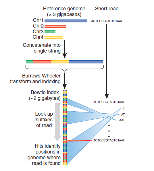
Figure 12.3: How Burrows-Wheeler indexing works
Burrows-Wheeler indexing takes the genome and scrambles it up in such a way such that you can look at the read one character at a time and throw out a huge chunk of the genome as possible alignment positions very quickly.
One major problem with these two general purpose alignment strategies is that they don’t account for large gaps in alignment.
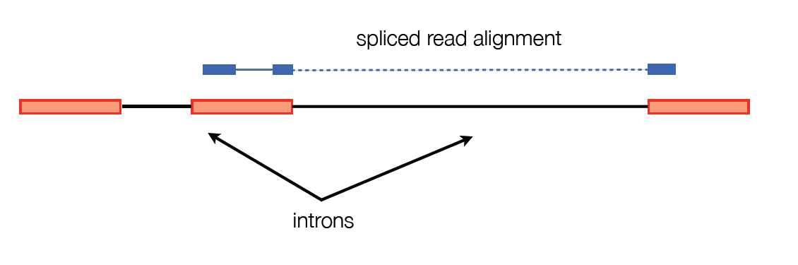
To get around this, TopHat breaks the reads into smaller pieces. These pieces are aligned and reads with pieces that are mapped far apart are flagged for possible intron sites. The pieces that weren’t able to be aligned are used to confirm the splice sites. The reads are then stitched back together to make full read alignments.
There are two strategies for assembling transcripts based on RNA-Seq reads.
1. Genome-guided approach (used in software such as Cufflinks)
The idea behind this approach is that we don’t necessarily know if two reads come from the same transcript, but we will know if they come from different transcripts. The algorithm is as follows: take the alignments and put them in a graph. Add an edge from x → y if x is to the left of y in the genome, x and y overlap consistently, and y is not contained in x. So we have an edge from x → y if they might come from the same transcript.
If we walk across this graph from left to right, we get a potential transcript. Applying Dilworth’s theorem to read partial orders, we can see that the size of the largest antichain in the graph is the minimum number of transcripts needed to explain the alignment. An antichain is a set of alignments with the property that no two are compatible (i.e. could arise from the same transcript)
2. Genome-independent approach (used in software such as trinity)
The genome-independent approach attempts to piece together the transcripts directly from the reads using classical methods for overlap based read assembly, similar to the genome assembly methods.
Calculating expression of genes and transcripts
We want to count the number of reads from each transcript to find the expression level of the transcript. However, since we divide transcripts into equally-sized fragments, we run into the problem that longer transcripts will naturally produce more reads than a shorter transcript. To account for this, we compute expression levels in FPKM, fragments per kilobase per million fragments mapped.
Likelihood function for a gene
Suppose we sequence a particular read, call it F1.
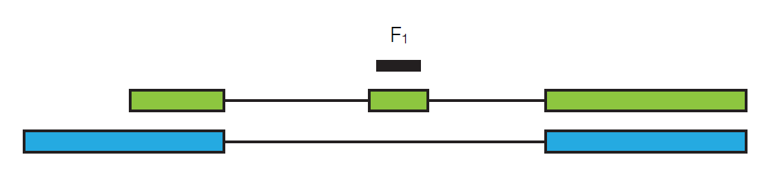
In order to get this particular read, we need to pick the particular transcript it’s in and then we need to pick this particular read out from the whole transcript. If we define \($\gamma_{\text {green }}$\) to be the relative abundance of the green transcript, then we have
\[P\left(F_{1} \mid \gamma_{\text {green }}\right)=\frac{\gamma_{\text {green }}}{l_{\text {green }}}\nonumber \]
where lgreen is the length of the green transcript. Now suppose we look at a different read, F2.
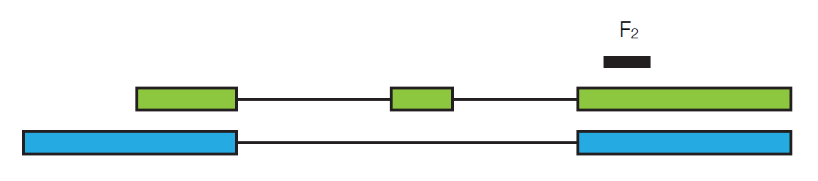
It could have come from either the green transcript of the blue transcript, so:
\[P\left(F_{2} \mid \gamma\right)=\frac{\gamma_{\text {green }}}{l_{\text {green }}}+\frac{\gamma_{\text {blue }}}{l_{\text {blue }}} \nonumber \]
We can see that the probability of getting both F1 and F2 is just the product of the individual probabilities:
\[P(F \mid \gamma)=\frac{\gamma_{\text {green }}}{l_{\text {green }}} \cdot\left(\frac{\gamma_{\text {green }}}{l_{\text {green }}}+\frac{\gamma_{\text {blue }}}{l_{\text {blue }}}\right) \nonumber \]
We define this as our likelihood function, L(F|γ). Given an input of abundances, we get a probability of how likely our sequence of reads is. So from a set of reads and transcripts, we can build a likelihood function and calculate the values for gamma that will maximize this function. Cufflinks achieves this using hill climbing or EM on the log-likelihood function.
Differential analysis with RNA-Seq
Suppose we perform an RNA-Seq analysis for a gene under two different conditions. How can we tell if there is a significant difference in the fragment counts? We calculate expression by estimating the expected number of fragments that come from each transcript. To test for significance, we need to know the variance of that estimate. We model the variance as:
Var(expression) = Technical variability + Biological variability
Technical variability, which is variability from uncertainty in mapping reads, can be modeled well with a Poisson distribution (see figure below). However, using Poisson to model biological variability, or variability across replicates, results in overdispersion.
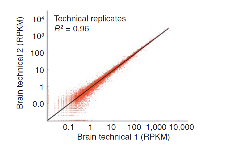
Figure 12.8: Technical variability follows a Poisson distribution
In the simple case where we have variability across replicates, but no uncertainty, we can mix the Poisson distributions from each replicate into a new distribution to model biological variability. We can treat the lambda parameter of the Poisson distribution as a random variable that follows a gamma distribution:
\[X \sim \operatorname{Poisson}(\Gamma(r, p)) \nonumber \]
The counts from this model follow a negative binomial distribution. To figure out the parameters for the negative binomial for each gene, we can fit a gamma function through a scatter plot of the mean count vs. count variance across replicates.
In the simple case where there is read mapping uncertainty, but not biological variability, we need to in- clude the mapping uncertainty in our variance estimate. Since we assign reads to transcripts probabilistically, we need to calculate the variance in that assignment.
The two threads of RNA-Seq expression analysis research focus on the problems in these two simple cases. One of the threads focuses on inferring the abundances of individual isoforms to learn about differential splicing and promoter use, while the other thread focuses on modeling variability across replicates to create more robust differential gene expression analysis. Cuffdiff unites these two separate threads to study the case where we have biological variability and read mapping ambiguity. Since overdispersion can be modeled with a negative binomial distribution and mapping uncertainty can be modeled with a Beta distribution, we combine these two to model this case with a beta negative binomial distribution.