10.7: Probabilistic Approach to the RNA Folding Problem

RNA-coding sequence inside the genome Finding RNA-coding sequences inside the genome is a very hard problem. However there are ways to do it. One way is to combine the thermodynamic stability information, with a normalized RNAfold score and then we can do a Support Vector Machine (SVM) classification, and compare the thermodynamic stability of the sequence to some random sequences of the same GC content and the same length and see how many standard deviations is the given structure more stable that the expected value.

We can combine it with the evolutionary measure and see if the RNA is more conserved or not. This gives us (with relative accuracy) an idea if the genomic sequence is actually coding an RNA.

We have studied only half of the story. Although the thermodynamic approach is a good way (and the classic way) of folding the RNAs, some part of the community like to study it from a different aspect. Lets assume for now that we don't

RNA-coding sequence inside the genome 

Finding RNA-coding sequences inside the genome is a very hard problem. However there are ways to do it. One way is to combine the thermodynamic stability information, with a normalized RNA fold score and then we can do a Support Vector Machine (SVM) classification, and compare the thermodynamic stability of the sequence to some random sequences of the same GC content and the same length and see how many standard deviations is the given structure more stable that the expected value.

know anything about the physics of RNA or the Boltzman factor. Instead, we look into the RNA as a string of letters for which we want to find the most probable structure. We have already learned about the Hidden Markov Models in the previous lectures. They are a nice way to make predictions about the hidden states of a probabilistic system. The question is can we use Hidden Markov models for the RNA folding problem? The answer is yes.

We can combine it with the evolutionary measure and see if the RNA is more conserved or not. This gives us (with relative accuracy) an idea if the genomic sequence is actually coding an RNA.

We have studied only half of the story. Although the thermodynamic approach is a good way (and the classic way) of folding the RNAs, some part of the community like to study it from a different aspect.

Lets assume for now that we don't know anything about the physics of RNA or the Boltzman factor. Instead, we look into the RNA as a string of letters for which we want to find the most probable structure. We have already learned about the Hidden Markov Models in the previous lectures. They are a nice way to make predictions about the hidden states of a probabilistic system. The question is can we use Hidden Markov models for the RNA folding problem? The answer is yes.

We can represent RNA structure as a set of hidden states of dots and brackets (recall the dot-bracket representation of RNA in part 3). There is an important observation to make here: the positions and the pairings inside the RNA are not independent, so we cannot simply have a state of an opening bracket without any considerations of the events that are happening downstream.

Therefore we need to extend the HMM framework to allow for nested correlations. Fortunately, the probabilistic framework to deal with such a problem already exists. It is known as stochastic context-free grammar (SCFG).

Context Free Grammar in a nutshell

You have:

• Finite set of non-terminal symbols (states) e.g. {A, B, C} and terminal symbols e.g. {a, b, c}
• Finite set of Production rules. e.g. {A → aB, B → AC, B → aa, → ab}
• An initial (start) nonterminal

You want to find a way to get from one state to another (or to a terminal). \[A→aB→aAC→ aaaC → aaaab \nonumber\]

In a stochastic CFG, the only difference is that each relation has a certain probability .e.g.: \[P(B → AC) = 0.25 P(B → aa) = 0.75 \nonumber\]

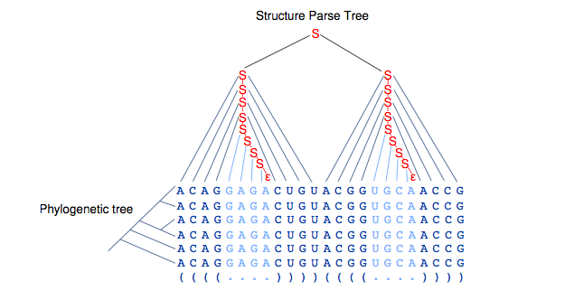
Phylogenetic evaluation is easily combined with SCFGs, since there are many probabilistic models for phylogenetic data. The Probabilistic models are not discussed in detail in this lecture but the following picture basically gives an analogy between the Stochastic models and the methods that we have see so far in the class.

• Analogies to thermodynamic folding:
  – CYK ↔ Minimum Free energy (Nussinov/Zuker)

  – Inside/outside algorithm ↔ Partition functions (McCaskill)

• Analogies to Hidden Markov models:

  – CYK Minimum ↔ Viterbi’s algorithm
  – Inside/outside algorithm ↔ Forward/backwards algorithm

• Given a parameterized SCFG (Θ,Ω) and a sequence x, the Cocke-Younger-Kasami (CYK) dynamic programming algorithm finds an optimal (maximum probability) parse tree \(\hat{\pi}\):

  \(\hat{\pi}\) = argmaxProb(π, x|Θ, Ω)

• The Inside algorithm, is used to obtain the total probability of the sequence given the model summed over all parse trees, \[\text{Prob}(x|Θ, Ω) = \sum \text{Prob}(x, π|Θ, Ω)\]

Application of SCFGs

• Consensus secondary structure prediction: Pfold – First Phylo-SCFG

Figure 10.14: A) Single sequence: Terminal symbols are bases or base-pairs, Emission probabilities are base frequencies in loops and paired regions B) Phylo-SCFG: Terminal symbols are single or paired alignment columns, Emission probabilities calculated from phylogenetic model and tree using Felsenstein’s algorithmWe to try to better understand RNA-RNA interactions. © Stefan Washietl. All rights reserved. This content is excluded from our Creative Commons license. For more information, see http://ocw.mit.edu/help/faq-fair-use/.

• Structural RNA gene nding: EvoFold

10.8

– Uses Pfold grammar
– Two competing models:

∗ Non-structural model with all columns treated as evolving independently

∗ Structural model with dependent and independent columns

– Sophisticated parametrization