8.2: Posterior Decoding

Motivation

Although the Viterbi decoding algorithm provides one means of estimating the hidden states underlying a sequence of observed characters, another valid means of inference is provided by posterior decoding.

Posterior decoding provides the most likely state at any point in time. To gain some intuition for posterior decoding, let’s see how it applies to the situation in which a dishonest casino alternates between a fair and loaded die. Suppose we enter the casino knowing that the unfair die is used 60 percent of the time. With this knowledge and no die rolls, our best guess for the current die is obviously the loaded one. After one roll, the probability that the loaded die was used is given by

\[\begin{equation}
P(\text {die}=\text {loaded} \mid \text {roll}=k)=\frac{P(\text {die}=\text {loaded}) * P(\text {roll}=k \mid \text {die}=\text {loaded})}{P(\text {roll}=k)}
\end{equation}\]

If we instead observed a sequence of N die rolls, how do perform a similar sort of inference? By allowing information to flow between the N rolls and influence the probability of each state, posterior decoding is a natural extension of the above inference to a sequence of arbitrary length. More formally, instead of identifying a single path of maximum likelihood, posterior decoding considers the probability of any path lying in state k at time t given all of the observed characters, i.e. P(πt = k|x₁,...,x_n). The state that maximizes this probability for a given time is then considered as the most likely state at that point.

It is important to note that in addition to information flowing forward to determine the most likely state at a point, information may also flow backward from the end of the sequence to that state to augment or reduce the likelihood of each state at that point. This is partly a natural consequence of the reversibility of Bayes’ rule: our probabilities change from prior probabilities into posterior probabilities upon observing more data. To elucidate this, imagine the casino example again. As stated earlier, without observing any rolls, the state0 is most likely to be unfair: this is our prior probability. If the first roll is a 6, our belief that state1 is unfair is reinforced (if rolling sixes is more likely in an unfair die). If a 6 is rolled again, information flow backwards from the second die roll and reinforces our state1 belief of an unfair die even more. The more rolls we have, the more information that flows backwards and reinforces or contrasts our beliefs about the state thus illustrating the way information flows backward and forward to affect our belief about the states in Posterior Decoding.

Using some elementary manipulations, we can rearrange this probability into the following form using Bayes’ rule:

\[\begin{equation}
\pi_{t}^{*}=\operatorname{argmax}_{k} P\left(\pi_{t}=k \mid x_{1}, \ldots, x_{n}\right)=\operatorname{argmax}_{k} \frac{P\left(\pi_{t}=k, x_{1}, \ldots, x_{n}\right)}{P\left(x_{1}, \ldots, x_{n}\right)}
\end{equation}\]

Because P (x) is a constant, we can neglect it when maximizing the function. Therefore,

\[\begin{equation}
\pi_{t}^{*}=\operatorname{argmax}_{k} P\left(\pi_{t}=k, x_{1}, \ldots, x_{t}\right) * P\left(x_{t+1}, \ldots, x_{n} \mid \pi_{t}=k, x_{1}, \ldots, x_{t}\right)
\end{equation}\]

Using the Markov property, we can simply write this expression as follows:

\[\begin{equation}
\pi_{t}^{*}=\operatorname{argmax}_{k} P\left(\pi_{t}=k, x_{1}, \ldots, x_{t}\right) * P\left(x_{t+1}, \ldots, x_{n} \mid \pi_{t}=k\right)=\operatorname{argmax}_{k} f_{k}(t) * b_{k}(t)
\end{equation}\]

Here, we’ve defined \(\begin{equation}
f_{k}(t)=P\left(\pi_{t}=k, x_{1}, \ldots, x_{t}\right) \text { and } b_{k}(t)=P\left(x_{t+1}, \ldots, x_{n} \mid \pi_{t}=k\right)
\end{equation}\). As we will shortly see, these parameters are calculated using the forward algorithm and the backward algorithm respectively. To solve the posterior decoding problem, we merely need to solve each of these subproblems. The forward algorithm has been illustrated in the previous chapter and in the review at the start of this chapter and the backward algorithm will be explained in the next section.

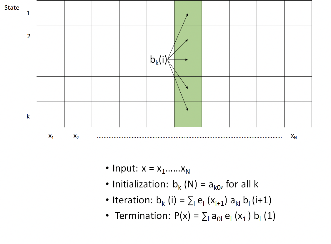
Backward Algorithm

As previously described, the backward algorithm is used to calculate the following probability:

\[\begin{equation}
b_{k}(t)=P\left(x_{t+1}, \ldots, x_{n} \mid \pi_{t}=k\right)
\end{equation}\]

We can begin to develop a recursion n by expanding into the following form:

\[\begin{equation}
b_{k}(t)=\sum_{l} P\left(x_{t+1}, \ldots, x_{n}, \pi_{t+1}=l \mid \pi_{t}=k\right)
\end{equation}\]

From the Markov property, we then obtain:

\[\begin{equation}
b_{k}(t)=\sum_{l} P\left(x_{t+2}, \ldots, x_{n} \mid \pi_{t+1}=l\right) * P\left(\pi_{t+1}=l \mid \pi_{t}=k\right) * P\left(x_{t+1} \mid \pi_{t+1}=k\right)
\end{equation}\]

The first term merely corresponds to bl(t+1). Expressing in terms of emission and transition probabilities gives the final recursion:

\[\begin{equation}
b_{k}(t)=\sum_{l} b_{l}(i+1) * a_{k l} * e_{l}\left(x_{t+1}\right)
\end{equation}\]

Comparison of the forward and backward recursions leads to some interesting insight. Whereas the forward algorithm uses the results at t − 1 to calculate the result for t, the backward algorithm uses the results from t + 1, leading naturally to their respective names. Another significant difference lies in the emission probabilities; while the emissions for the forward algorithm occur from the current state and can therefore be excluded from the summation, the emissions for the backward algorithm occur at time t + 1 and therefore must be included within the summation.

Given their similarities, it is not surprising that the backward algorithm is also implemented using a KxN dynamic programming table. The algorithm, as depicted in Figure 8.3, begins by initializing the rightmost column of the table to unity. Proceeding from right to left, each column is then calculated by taking a weighted sum of the values in the column to the right according to the recursion outlined above. After calculating the leftmost column, all of the backward probabilities have been calculated and the algorithm terminates. Because there are KN entries and each entry examines a total of K other entries, this leads to O(K²N) time complexity and O(KN) space, bounds identical to those of the forward algorithm.

Just as P(X) was calculated by summing the rightmost column of the forward algorithm’s DP table, P(X) can also be calculated from the sum of the leftmost column of the backward algorithm’s DP table. Therefore, these methods are virtually interchangeable for this particular calculation.

Figure 8.3: The Backward Algorithm

Did You Know?

Note that even when executing the backward algorithm, forward transition probabilities are used i.e if moving in the backward direction involves a transition from state B → A, the probability of transitioning from state A → B is used. This is because moving backward from state B to state A implies that state B follows state A in our normal, forward order, thus calling for the same transition probability.

The Big Picture

Why do we have to make both forward and backward calculations for posterior decoding, while the algorithms that we have discussed previously call for only one direction? The difference lies in the fact that posterior decoding seeks to produce probabilities for the underlying states of individual positions rather than whole sequences of positions. In seeking to find the most likely underlying state of a given position, we need to take into account the entire sequence in which that position exists, both before and after it, as befits a Bayesian approach - and to do this in a dynamic programming algorithm, in which we compute recursively and end with a maximizing function, we must approach our position of interest from both sides.

Given that we can calculate both f_k(t) and b_k(t) in θ(K²N) time and θ(KN) space for all t = 1 . . . n, we can use posterior decoding to determine the most likely state π_t^∗ for t = 1 . . . n. The relevant expression is given by

\[\begin{equation}
\pi_{t}^{*}=\operatorname{argmax}_{k} P\left(\pi_{i}=k \mid x\right)=\frac{f_{k}(i) * b_{k}(i)}{P(x)}
\end{equation}\]

With two methods (Viterbi and posterior) to decode, which is more appropriate? When trying to classify each hidden state, the Posterior decoding method is more informative because it takes into account all possible paths when determining the most likely state. In contrast, the Viterbi method only takes into account one path, which may end up representing a minimal fraction of the total probability. At the same time, however, posterior decoding may give an invalid sequence of states! By selecting for the maximum probability state of each position independently, we’re not considering how likely the transitions between these states are. For example, the states identified at time points t and t + 1 might have zero transition probability between them. As a result, selecting a decoding method is highly dependent on the application of interest.

FAQ

Q: What does it imply when the Viterbi algorithm and Posterior decoding disagree on the path?

A: In a sense, it is simply a reminder that our model gives us what it’s selecting for. When we seek the maximum probability state of each independent position and disregard transitions between these max probability states, we may get something different than when we seek to find the most likely total path. Biology is complicated; it is important to think about what metric is most relevant to the biological situation at hand. In the genomic context, a disagreement might be a result of some ’funky’ biology; alternative splicing, for instance. In some cases, the Viterbi algorithm will be close to the Posterior decoding while in some others they may disagree.