8.1: Review of previous lecture

Introduction to Hidden Markov Models

In the last lecture, we familiarized ourselves with the concept of discrete-time Markov chains and Hidden Markov Models (HMMs). In particular, a Markov chain is a discrete random process that abides by the Markov property, i.e. that the probability of the next state depends only on the current state; this property is also frequently called ”memorylessness.” To model how states change from step to step, the Markov chain uses a matrix of transition probabilities. In addition, it is characterized by a one-to-one correspondence between the states and observed symbols; that is, the state fully determines all relevant observables. More formally, a Markov chain is fully defined by the following variables:

• π_i ∈ Q, the state at the i^th step in a sequence of finite states Q of length N that can hold a value from a finite alphabet Σ of length K

• a_jk, the transition probability of moving from state j to state k, P(π_i = k|π_i−1 = j), for each j,k in Q

• a_0j ∈ P , the probability that the initial state will be j

Examples of Markov chains are abundant in everyday life. In the last lecture, we considered the canonical example of a weather system in which each state is either rain, snow, sun or clouds and the observables of the system correspond exactly to the underlying state: there is nothing that we don’t know upon making an observation, as the observation, i.e. whether it is sunny or raining, fully determines the underlying state, i.e. whether it is sunny or raining. Suppose, however, that we are considering the weather as it is probabilistically determined by the seasons - for example, it snows more often in the winter than in the spring - and suppose further that we are in ancient times and did not yet have access to knowledge about what the current season is. Now consider the problem of trying to infer the season (the hidden state) from the weather (the observable). There is some relationship between season and weather such that we can use information about the weather to make inferences about what season it is (if it snows a lot, it’s probably not summer); this is the task that HMMs seek to undertake. Thus, in this situation, the states, the seasons, are considered “hidden” and no longer share a one-to-one correspondence with the observables, the weather. These types of situations require a generalization of Markov chains known as Hidden Markov Models (HMMs).

Did You Know?

Markov Chains may be thought of as WYSIWYG - What You See Is What You Get

HMMs incorporate additional elements to model the disconnect between the observables of a system and the hidden states. For a sequence of length N, each observable state is instead replaced by a hidden state (the season) and a character emitted from that state (the weather). It is important to note that characters from each state are emitted according to a series of emission probabilities (say there is a 50% chance of snow, 30% chance of sun, and 20% chance of rain during winter). More formally, the two additional descriptors of an HMM are:

• x_i ∈ X, the emission at the i^th step in a sequence of finite characters X of length N that can hold a character from a finite set of observation symbols v_l ∈ V
• e_k(v_l) ∈ E, the emission probability of emitting character vl when the state is k, P(x_i = v_l|π_i = k) In summary, an HMM is defined by the following variables:

• a_jk, e_k(v_l), and a_0j that model the discrete random process
• π_i, the sequence of hidden states
• x_i, the sequence of observed emissions

Genomic Applications of HMMs

The figure below shows some genomic applications of HMMs

Figure 8.1: Genomic applications of HMMs

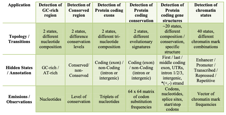
Niceties of some of the applications shown in figure 8.1 include:

• Detection of Protein coding conservation
This is similar to the application of detecting protein coding exons because the emissions are also not nucleotides but different in the sense that, instead of emitting codons, substitution frequencies of the codons are emitted.

• Detection of Protein coding gene structures
Here, it is important for different states to model first, last and middle exons independently, because they have distinct relevant structural features: for example, the first exon in a transcript goes through a start codon, the last exon goes through a stop codon, etc., and to make the best predictions, our model should encode these features. This differs from the application of detecting protein coding exons because in this case, the position of the exon is unimportant.
It is also important to differentiate between introns 1,2 and 3 so that the reading frame between one exon and the next exon can be remembered e.g. if one exon stops at the second codon position, the next one has to start at the third codon position. Therefore, the additional intron states encode the codon position.

• Detection of chromatin states
Chromatin state models are dynamic and vary from cell type to cell type so every cell type will have its own annotation. They will be discussed in fuller detail in the genomics lecture including strategies for stacking/concatenating cell types.

Viterbi decoding

Previously, we demonstrated that when given a full HMM (Q,A,X,E,P), the likelihood that the discrete random process produced the provided series of hidden states and emissions is given by:

\[P\left(x_{1}, \ldots, x_{N}, \pi_{1}, \ldots, \pi_{N}\right)=a_{0 \pi_{i}} \prod_{i} e_{\pi_{i}}\left(x_{i}\right) a_{\pi_{i} \pi_{i+1}}\]

This corresponds to the total joint probability, P(x,π). Usually, however, the hidden states are not given and must be inferred; we’re not interested in knowing the probability of the observed sequence given an underlying model of hidden states, but rather want to us the observed sequence to infer the hidden states, such as when we use an organism’s genomic sequence to infer the locations of its genes. One solution to this decoding problem is known as the Viterbi decoding algorithm. Running in O(K²N) time and O(KN) space, where K is the number of states and N is the length of the observed sequence, this algorithm determines the sequence of hidden states (the path π^∗) that maximizes the joint probability of the observables and states, i.e. P(x,π). Essentially, this algorithm defines V_k(i) to be the probability of the most likely path ending at state π_i = k, and it utilizes the optimal substructure argument that we saw in the sequence alignment module of the course to recursively compute V_k(i) = e_k(xi) × max_j(V_j(i − 1)a_jk) in a dynamic programming algorithm.

Forward Algorithm

Returning for a moment to the problem of ’scoring’ rather than ’decoding,’ another problem that we might want to tackle is that of, instead of computing the probability of a single path of hidden state emitting the observed sequence, calculating the total probability of the sequence being produced by all possible paths. For example, in the casino example, if the sequence of rolls is long enough, the probability of any single observed sequence and underlying path is very low, even if it is the single most likely sequence-path combination. We may instead want to take an agnostic attitude toward the path and assess the total probability of the observed sequence arising in any way.

In order to do that, we proposed the Forward algorithm, which is described in Figure 8.2

Figure 8.2: The Forward Algorithm

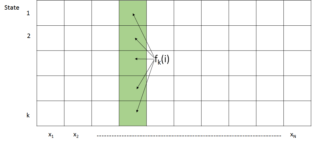
\[\begin{equation}
\begin{array}{l}
\text { Input: } x=x_{1} \ldots x_{N} \\
\text { Initialization: } \\
\qquad f_{0}(0)=1, f_{k}(0)=0, \quad \text { for all } k>0 \\
\text { Iteration: } \\
\qquad f_{k}(i)=e_{k}\left(x_{i}\right) \times \sum_{j} a_{j k} f_{j}(i-1)
\end{array}
\end{equation} \nonumber \]

\[\text {Termination:} \\ \begin{equation}
P\left(x, \pi^{*}\right)=\sum_{k} f_{k}(N)
\end{equation} \nonumber \]

The forward algorithm first calculates the joint probability of observing the first t emitted characters and being in state k at time t. More formally,
\[\begin{equation}
f_{k}(t)=P\left(\pi_{t}=k, x_{1}, \ldots, x_{t}\right)
\end{equation}\]

Given that the number of paths is exponential in t, dynamic programming must be employed to solve this problem. We can develop a simple recursion for the forward algorithm by employing the Markov property as follows:

\[\begin{equation}
f_{k}(t)=\sum_{l} P\left(x_{1}, \ldots, x_{t}, \pi_{t}=k, \pi_{t-1}=l\right)=\sum_{l} P\left(x_{1}, \ldots, x_{t-1}, \pi_{t-1}=l\right) * P\left(x_{t}, \pi_{t} \mid \pi_{t-1}\right)
\end{equation}\]

Recognizing that the first term corresponds to fl(t − 1) and that the second term can be expressed in terms of transition and emission probabilities, this leads to the final recursion:

\[\begin{equation}
f_{k}(t)=e_{k}\left(x_{t}\right) \sum_{l} f_{l}(t-1) * a_{l k}
\end{equation}\]

Intuitively, one can understand this recursion as follows: Any path that is in state k at time t must have come from a path that was in state l at time t − 1. The contribution of each of these sets of paths is then weighted by the cost of transitioning from state l to state k. It is also important to note that the Viterbi algorithm and forward algorithm largely share the same recursion. The only difference between the two algorithms lies in the fact that the Viterbi algorithm, seeking to find only the single most likely path, uses a maximization function, whereas the forward algorithm, seeking to find the total probability of the sequence over all paths, uses a sum.

We can now compute f_k(t) based on a weighted sum of all the forward algorithm results tabulated during the previous time step. As shown in Figure 8.2, the forward algorithm can be easily implemented in a KxN dynamic programming table. The first column of the table is initialized according to the initial state probabilities a_i0 and the algorithm then proceeds to process each column from left to right. Because there are KN entries and each entry examines a total of K other entries, this leads to O(K²N) time complexity and O(KN) space.

In order now to calculate the total probability of a sequence of observed characters under the current HMM, we need to express this probability in terms of the forward algorithm gives in the following way:

\[\begin{equation}
P\left(x_{1}, \ldots, x_{n}\right)=\sum_{l} P\left(x_{1}, \ldots, x_{n}, \pi_{N}=l\right)=\sum_{l} f_{l}(N)
\end{equation}\]

Hence, the sum of the elements in the last column of the dynamic programming table provides the total probability of an observed sequence of characters. In practice, given a sufficiently long sequence of emitted characters, the forward probabilities decrease very rapidly. To circumvent issues associated with storing small floating point numbers, logs-probabilities are used in the calculations instead of the probabilities themselves. This alteration requires a slight adjustment to the algorithm and the use of a Taylor series expansion for the exponential function.

This lecture

• This lecture will discuss posterior decoding, an algorithm which again will infer the hidden state sequence π that maximizes a different metric. In particular, it finds the most likely state at every position over all possible paths and does so using both the forward and backward algorithm.
• Afterwards, we will show how to encode “memory” in a Markov chain by adding more states to search a genome for dinucleotide CpG islands.
• We will then discuss how to use Maximum Likelihood parameter estimation for supervised learning with a labelled dataset
• We will also briefly see how to use Viterbi learning for unsupervised estimation of the parameters of an unlabelled dataset
• Finally, we will learn how to use Expectation Maximization (EM) for unsupervised estimation of parameters of an unlabelled dataset where the specific algorithm for HMMs is known as the Baum- Welch algorithm.