7.4: Apply HMM to Real World- From Casino to Biology
- Page ID
- 40955

The Dishonest Casino
Imagine the following scenario: You enter a casino that offers a dice-rolling game. You bet $1 and then you and a dealer both roll a die. If you roll a higher number you win $2. Now there’s a twist to this seemingly simple game. You are aware that the casino has two types of dice:
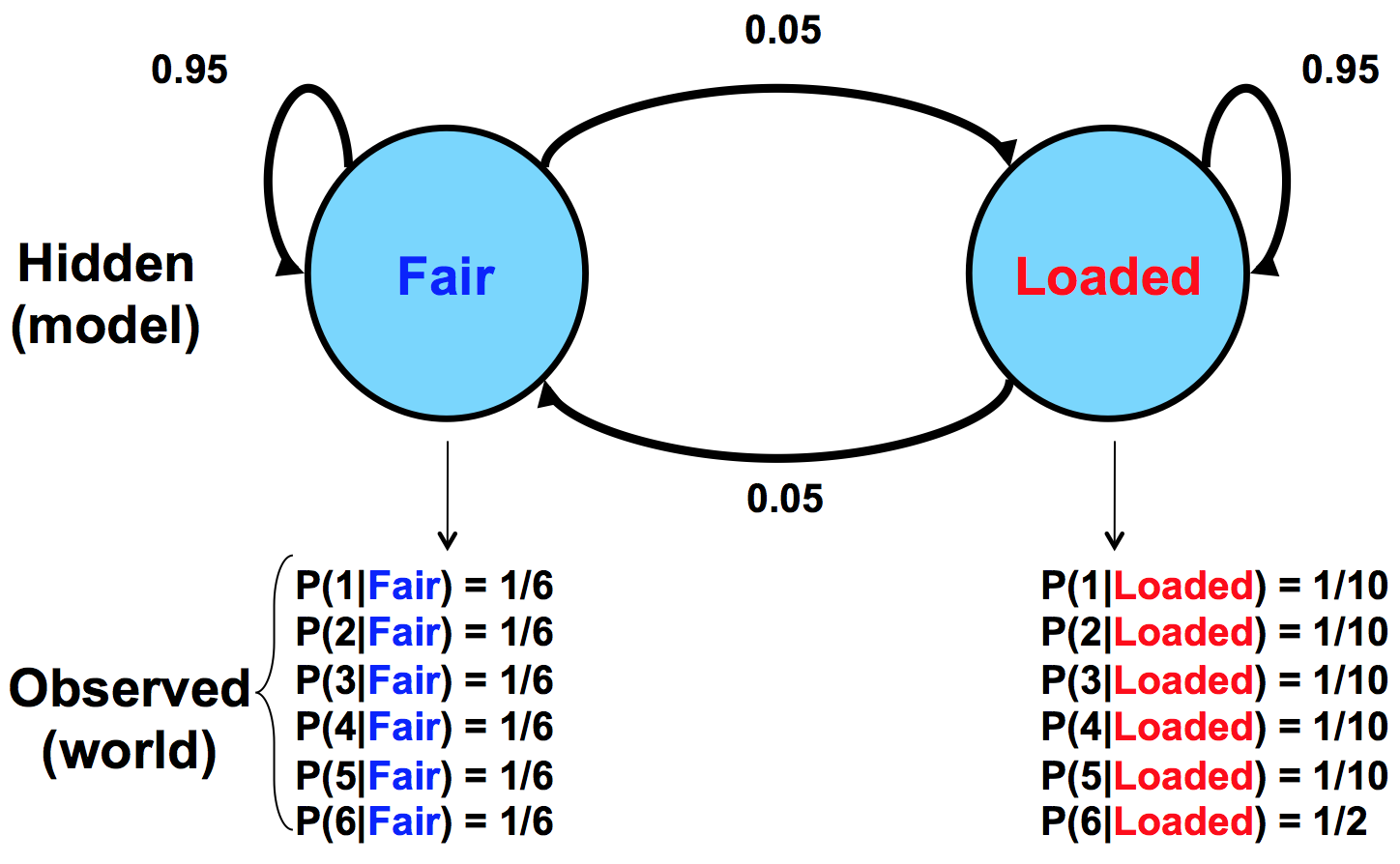
- Fair die: P(1)=P(2)=P(3)=P(4)=P(5)=P(6)=1/6
- Loaded die: P(1) = P(2) = P(3) = P(4) = P(5) = 1/10 and P(6) = 1/2
The dealer can switch between these two dice at any time without you knowing it. The only information that you have are the rolls that you observe. We can represent the state of the casino die with a simple Markov model:
The model shows the two possible states, their emissions, and probabilities for transition between them. The transition probabilities are educated guesses at best. We assume that switching between the states doesn’t happen too frequently, hence the .95 chance of staying in the same state with every roll.
Staying in touch with biology: An analogy
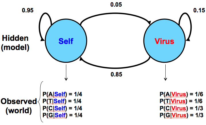
For comparison, Figure 7.5 below gives a similar model for a situation in biology where a sequence of DNA has two potential sources: injection by a virus versus normal production by the organism itself:
Given this model as a hypothesis, we would observe the frequencies of C and G to give us clues as to the source of the sequence in question. This model assumes that viral inserts will have higher CpG prevalence, which leads to the higher probabilities of C and G occurrence.
Running the Model
Say we are at the casino and observe the sequence of rolls given in Figure 7.6. We would like to know whether it is more likely that the casino is using the fair die or the loaded die.

Let’s look at a particular sequence of rolls.
Therefore, we will consider two possible sequences of states in the underlying HMM, one in which the dealer is always using a fair die, and the other in which the dealer is always using a loaded die. We consider each execution path to understand the implications. For each case, we compute the joint probability of an observed outcome with that sequence of underlying states.
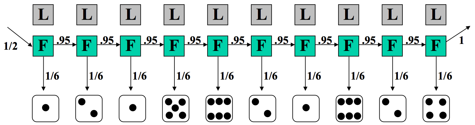
In the first case, where we assume the dealer is always using a fair die, the transition and emission probabilities are shown in Figure 7.7. The probability of this sequence of states and observed emissions is a product of terms which can be grouped into three components: 1/2, the probability of starting with the fair die; (1/6)10, the probability of the sequence of rolls if we always use the fair die; and lastly (0.95)9, the probability that we always continue to use the fair die.
In this model, we assume \(π = {F,F,F,F,F,F,F,F,F,F}\), and we observe \(x = {1,2,1,5,6,2,1,6,2,4}\).
Now we can calculate the joint probability of x and π as follows:
\[\begin{aligned}
P(x, \pi) &=P(x \mid \pi) P(\pi) \\
&=\frac{1}{2} \times P(1 \mid F) \times P(F \mid F) \times P(2 \mid F) \cdots \\
&=\frac{1}{2} \times\left(\frac{1}{6}\right)^{10} \times(0.95)^{9} \\
&=5.2 \times 10^{-9}
\end{aligned}\nonumber \]
With a probability this small, this might appear to be an extremely unlikely case. In actuality, the probability is low because there are many equally likely possibilities, and no one outcome is a priori likely. The question is not whether this sequence of hidden states is likely, but whether it is more likely than the alternatives.
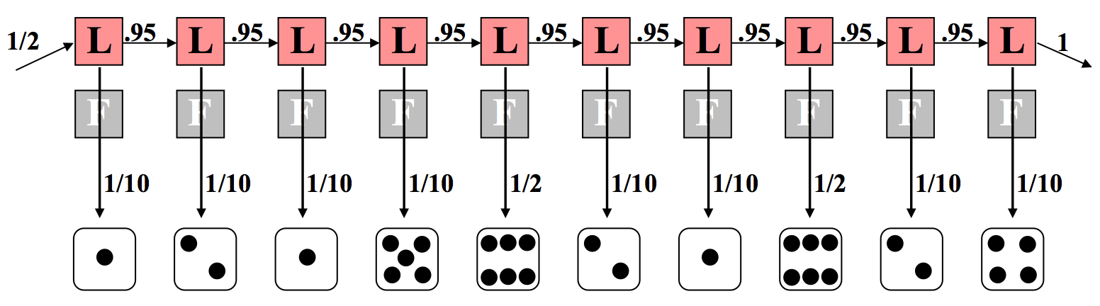
Let us consider the opposite extreme where the dealer always uses a loaded die, as depicted in Figure 7.8. This has a similar calculation except that we note a difference in the emission component. This time, 8 of the 10 rolls carry a probability of 1/10 because the loaded die disfavors non-sixes. The remaining two rolls of six have each a probability of 1/2 of occurring. Again we multiply all of these probabilities together according to principles of independence and conditioning. In this case, the calculations are as follows:
\[ \begin{align*}
P(x, \pi) &=\frac{1}{2} \times P(1 \mid L) \times P(L \mid L) \times P(2 \mid L) \cdots \\
&=\frac{1}{2} \times\left(\frac{1}{10}\right)^{8} \times\left(\frac{1}{2}\right)^{2} \times(0.95)^{9} \\
&=7.9 \times 10^{-10}
\end{align*}\]
Note the difference in exponents. If we make a direct comparison, we can say that the situation in which a fair die is used throughout the sequence is 52 × 10−10 (as compared with 7.9 × 10⁻¹⁰ with the loaded die).
Therefore, it is six times more likely that the fair die was used than that the loaded die was used. This is not too surprising—two rolls out of ten yielding a 6 is not very far from the expected number 1.7 with the fair die, and farther from the expected number 5 with the loaded die.
Adding Complexity
Now imagine the more complex, and interesting, case where the dealer switches the die at some point during the sequence. We make a guess at an underlying model based on this premise in Figure 7.9.
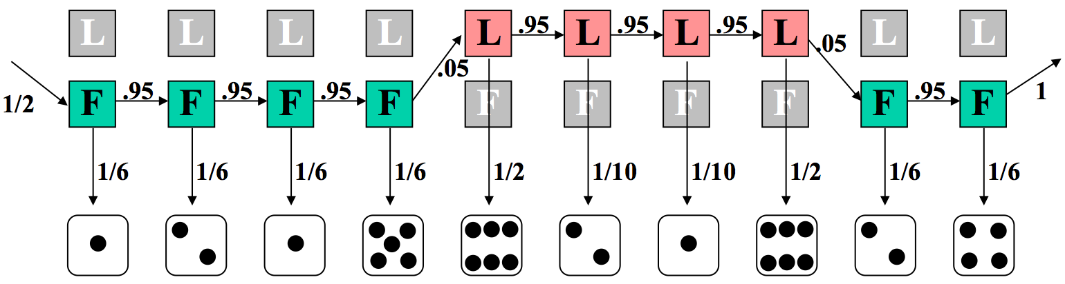
Again, we can calculate the likelihood of the joint probability of this sequence of states and observations. Here, six of the rolls are calculated with the fair die, and four with the loaded one. Additionally, not all of the transition probabilities are 95% anymore. The two swaps (between fair and loaded) each have a probability of 5%.
\[ \begin{aligned}
P(x, \pi) &=\frac{1}{2} \times P(1 \mid L) \times P(L \mid L) \times P(2 \mid L) \cdots \\
&=\frac{1}{2} \times\left(\frac{1}{10}\right)^{2} \times\left(\frac{1}{2}\right)^{2} \times\left(\frac{1}{6}\right)^{6} \times(0.95)^{7} \times(0.05)^{2} \\
&=4.67 \times 10^{-11}
\end{aligned} \nonumber \]
Back to Biology
Now that we have formalized HMMs, we want to use them to solve some real biological problems. In fact, HMMs are a great tool for gene sequence analysis, because we can look at a sequence of DNA as being emitted by a mixture of models. These may include introns, exons, transcription factors, etc. While we may have some sample data that matches models to DNA sequences, in the case that we start fresh with a new piece of DNA, we can use HMMs to ascribe some potential models to the DNA in question. We will first introduce a simple example and think about it a bit. Then, we will discuss some applications of HMM in solving interesting biological questions, before finally describing the HMM techniques that solve the problems that arise in such a first-attempt/native analysis.
A simple example: Finding GC-rich regions
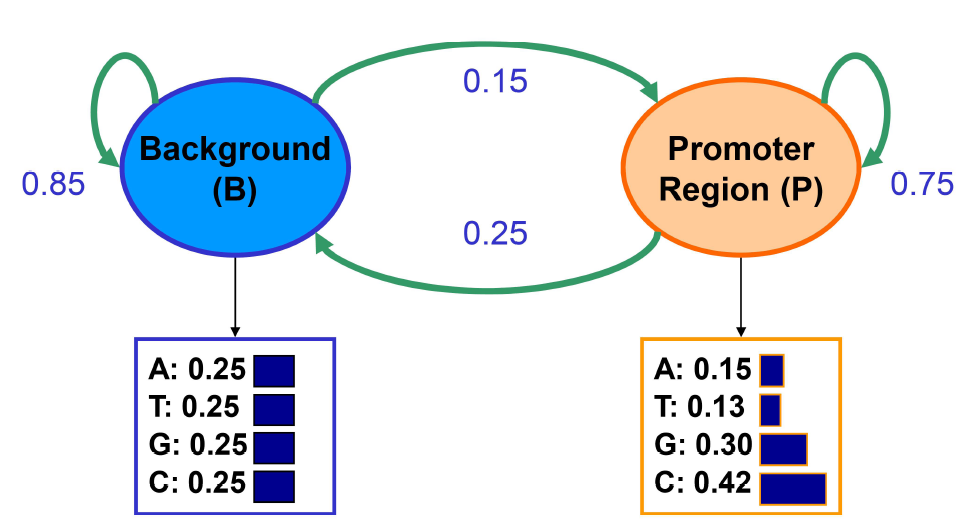
Imagine the following scenario: we are trying to find GC rich regions by modeling nucleotide sequences drawn from two different distributions: background and promoter. Background regions have uniform distribution of 0.25 for each of A, T, G, C. Promoter regions have probabilities: A: 0.15, T: 0.13, G: 0.30, C: 0.42. Given one nucleotide observed, we cannot say anything about the region from which it was originated, because either region will emit each nucleotide at some probability. We can learn these initial state probabilities based in steady state probabilities. By looking at a sequence, we want to identify which regions originate from a background distribution (B) and which regions are from a promoter model (P).
We are given the transition and emission probabilities based on relevant abundance and average length of regions where x = vector of observable emissions consisting of symbols from the alphabet {A,T,G,C}; π = vector of states in a path (e.g. BPPBP); π∗ = maximum likelihood of generating that path. In our interpretation of sequence, the max likelihood path will be found by incorporating all emission and transition probabilities by dynamic programming.
HMMs are generative models, in that an HMM gives the probability of emission given a state (using Bayes’ Rule), essentially telling you how likely the state is to generate those sequences. So we can always run a generative model for transitions between states and start anywhere. In Markov Chains, the next state will give different outcomes with different probabilities. No matter which state is next, at the next state, the next symbol will still come out with different probabilities. HMMs are similar: You can pick an initial state based on the initial probability vector. In the example above, we will start in state B with high probability since most locations do not correspond to promoter regions. You then draw an emission from the P(X|B). Each nucleotide occurs with probability 0.25 in the background state. Say the sampled nucleotide is a G. The distribution of subsequent states depends only on the fact that we are in the background state and is independent of this emission. So we have that the probability of remaining in state B is 0.85 and the probability of transitioning to state P is 0.15, and so on.
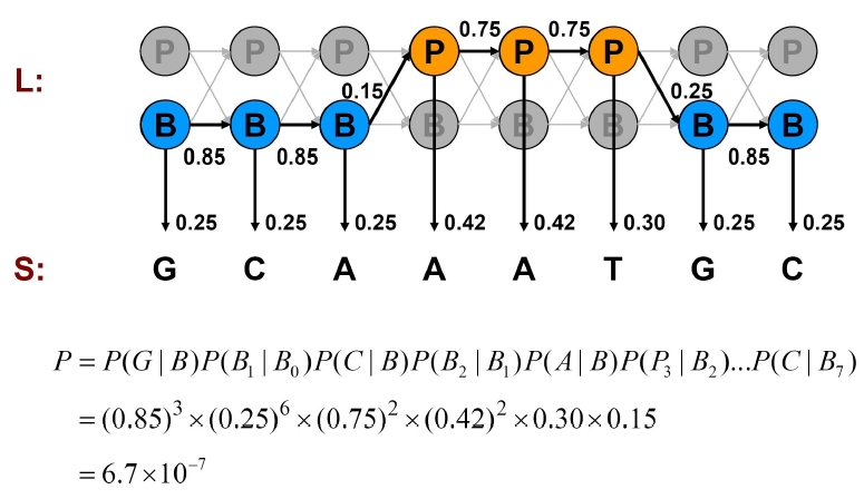
We can compute the probability of one such generation by multiplying the probabilities that the model makes exactly the choices we assumed. Consider the examples shown in Figures 7.11, 7.12, and 7.13.
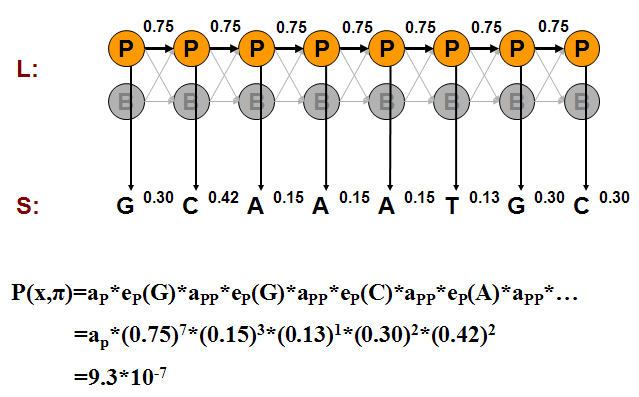
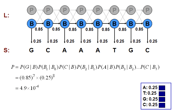
We can calculate the joint probability of a particular sequence of states corresponding to the observed emissions as we did in the Casino examples:
\[ \begin{aligned}
P\left(x, \pi_{P}\right) &=a_{P} \times e_{P}(G) \times a_{P P} \times e_{P}(G) \times \cdots \\
&=a_{P} \times(0.75)^{7} \times(0.15)^{3} \times(0.13) \times(0.3)^{2} \times(0.42)^{2} \\
&=9.3 \times 10^{-7} \\
P\left(x, \pi_{B}\right) &=(0.85)^{7} \times(0.25)^{8} \\
&=4.9 \times 10^{-6} \\
P\left(x, \pi_{\text {mixed}}\right) &=(0.85)^{3} \times(0.25)^{6} \times(0.75)^{2} \times(0.42)^{2} \times 0.3 \times 0.15 \\
&=6.7 \times 10^{-7}
\end{aligned} \nonumber \]
The pure-background alternative is the most likely option of the possibilities we have examined. But how do we know whether it is the option most likely out of all possibile paths of states to have generated the observed sequence?
The brute force approach is to examine at all paths, trying all possibilities and calculating their joint probabilities P(x,π) as we did above. The sum of probabilities of all the alternatives is 1. For example, if all states are promoters, \( P(x, \pi)=9.3 \times 10^{-7} \). If all emissions are Gs, \(P(x, \pi)=4.9 \times 10^{-6}\). the mixture of B’s and P ’s as in Figure 7.13, P (x, π) = 6.7 × 10⁻⁷; which is small because a lot of penalty is paid for the transitions between B’s and P’s which are exponential in length of sequence. Usually, if you observe more G’s, it is more likely to be in the promoter region and if you observe more A and Ts, then it is more likely to be in the background. But we need something more than just observation to support our belief. We will see how can we mathematically support our intuition in the following sections.
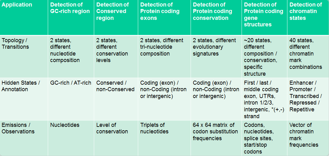
Application of HMMs in Biology
HMMs are used in answering many interesting biological questions. Some biological application of HMMs are summarized in Figure 7.14.