
3.3: Global alignment vs. Local alignment vs. Semi-global alignment
- Page ID
- 40922

A global alignment is defined as the end-to-end alignment of two strings s and t.
A local alignment of string s and t is an alignment of substrings of s with substrings of t.
In general are used to find regions of high local similarity. Often, we are more interested in finding local
alignments because we normally do not know the boundaries of genes and only a small domain of the gene may be conserved. In such cases, we do not want to enforce that other (potentially non-homologous) parts of the sequence also align. Local alignment is also useful when searching for a small gene in a large chromosome or for detecting when a long sequence may have been rearranged (Figure 4).
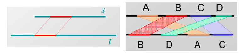
A semi-global alignment of string s and t is an alignment of a substring of s with a substring of t.
This form of alignment is useful for overlap detection when we do not wish to penalize starting or ending gaps. For finding a semi-global alignment, the important distinctions are to initialize the top row and leftmost column to zero and terminate end at either the bottom row or rightmost column.
The algorithm is as follows:
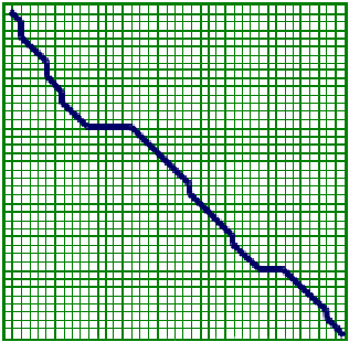
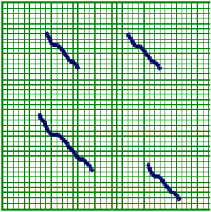
Figure 3.3: Local Alignment
\[
\begin{array}{l}
\text { Initialization } : \begin{aligned}
F(i, 0)=0 \\
F(0, j)=0
\end{aligned} \\
\qquad \begin{aligned}
\text {Iteration} : & F(i, j)=\max \left\{\begin{aligned}
F(i-1, j)-d \\
F(i, j-1)-d & \\
F(i-1, j-1)+s\left(x_{i}, y_{j}\right)
\end{aligned}\right.
\end{aligned}
\end{array}
\]
\[\text{Termination : Bottom row or Right column} \nonumber \]
Using Dynamic Programming for local alignments
In this section we will see how to find local alignments with a minor modification of the Needleman-Wunsch algorithm that was discussed in the previous chapter for finding global alignments.
To find global alignments, we used the following dynamic programming algorithm (Needleman-Wunsch algorithm):
\[ \text {Initialization : F(0,0)=0} \nonumber \]
\[\begin{aligned} \text { Iteration } &: F(i, j)=\max \left\{\begin{aligned} F(i-1, j)-d \\ F(i, j-1)-d \\ F(i-1, j-1)+s\left(x_{i}, y_{j}\right) \end{aligned}\right.\end{aligned}\]
\[\text{Termination : Bottom right} \nonumber \]
For finding local alignments we only need to modify the Needleman-Wunsch algorithm slightly to start over and find a new local alignment whenever the existing alignment score goes negative. Since a local alignment can start anywhere, we initialize the first row and column in the matrix to zeros. The iteration step is modified to include a zero to include the possibility that starting a new alignment would be cheaper than having many mismatches. Furthermore, since the alignment can end anywhere, we need to traverse the entire matrix to find the optimal alignment score (not only in the bottom right corner). The rest of the algorithm, including traceback, remains unchanged, with traceback indicating an end at a zero, indicating the start of the optimal alignment.
These changes result in the following dynamic programming algorithm for local alignment, which is also known as the :
\[ \begin{array}{ll}
\text { Initialization }: & F(i, 0)=0 \\
& F(0, j)=0
\end{array} \nonumber \]
\[\text {Iteration}: \quad F(i, j)=\max \left\{\begin{array}{c}
0 \\
F(i-1, j)-d \\
F(i, j-1)-d \\
F(i-1, j-1)+s\left(x_{i}, y_{j}\right)
\end{array}\right. \nonumber \]
\[ Termination : Anywhere \nonumber \]
Algorithmic Variations
Sometimes it can be costly in both time and space to run these alignment algorithms. Therefore, this section presents some algorithmic variations to save time and space that work well in practice.
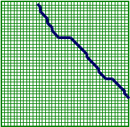
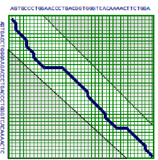
One method to save time, is the idea of bounding the space of alignments to be explored. The idea is that good alignments generally stay close to the diagonal of the matrix. Thus we can just explore matrix cells within a radius of k from the diagonal. The problem with this modification is that this is a heuristic and can lead to a sub-optimal solution as it doesn’t include the boundary cases mentioned at the beginning of the chapter. Nevertheless, this works very well in practice. In addition, depending on the properties of the scoring matrix, it may be possible to argue the correctness of the bounded-space algorithm. This algorithm requires \( O(k ∗ m) \) space and \( O(k ∗ m) \) time.
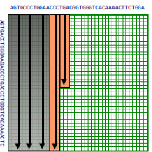
We saw earlier that in order to compute the optimal solution, we needed to store the alignment score in each cell as well as the pointer reflecting the optimal choice leading to each cell. However, if we are only interested in the optimal alignment score, and not the actual alignment itself, there is a method to compute the solution while saving space. To compute the score of any cell we only need the scores of the cell above, to the left, and to the left-diagonal of the current cell. By saving the previous and current column in which we are computing scores, the optimal solution can be computed in linear space.
If we use the principle of divide and conquer, we can actually find the optimal alignment with linear space. The idea is that we compute the optimal alignments from both sides of the matrix i.e. from the left to the right, and vice versa. Let \( u=\left\lfloor\frac{n}{2}\right\rfloor \). Say we can identify v such that cell \( (u, v) \) is on the optimal
© source unknown. All rights reserved. This content is excluded from our Creative Commons license. For more information, see http://ocw.mit.edu/help/faq-fair-use/.
alignment path. That means v is the row where the alignment crosses column u of the matrix. We can find the optimal alignment by concatenating the optimal alignments from (0,0) to (u,v) plus that of (u,v) to (m, n), where m and n is the bottom right cell (note: alignment scores of concatenated subalignments using our scoring scheme are additive. So we have isolated our problem to two separate problems in the the top left and bottom right corners of the DP matrix. Then we can recursively keep dividing up these subproblems to smaller subproblems, until we are down to aligning 0-length sequences or our problem is small enough to apply the regular DP algorithm. To find v the row in the middle column where the optimal alignment crosses we simply add the incoming and outgoing scores for that column.
One drawback of this divide-and-conquer approach is that it has a longer runtime. Nevertheless, the runtime is not dramatically increased. Since v can be found using one pass of regular DP, we can find v for each column in \( O(mn) \) time and linear space since we don’t need to keep track of traceback pointers for this step. Then by applying the divide and conquer approach, the subproblems take half the time since we only need to keep track of the cells diagonally along the optimal alignment path (half of the matrix of the previous step) That gives a total run time of \( O\left(m n\left(1+\frac{1}{2}+\frac{1}{4}+\ldots\right)\right)=O(2 M N)=O(m n) \) (using the sum of geometric series), to give us a quadratic run time (twice as slow as before, but still same asymptotic behavior). The total time will never exceed \( 2MN \) (twice the time as the previous algorithm). Although the runtime is increased by a constant factor, one of the big advantages of the divide-and-conquer approach is that the space is dramatically reduced to \( O(N) \).
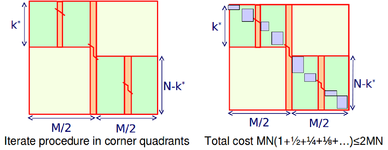
Figure 3.9: Divide and Conquer
Q: Why not use the bounded-space variation over the linear-space variation to get both linear time and linear space?
A: The bounded-space variation is a heuristic approach that can work well in practice but does not guarantee the optimal alignment.
Generalized gap penalties
Gap penalties determine the score calculated for a subsequence and thus affect which alignment is selected. The normal model is to use a where each individual gap in a sequence of gaps of length k is penalized equally with value p. This penalty can be modeled as \( w(k) = k ∗ p \). Depending on the situation, it could be a good idea to penalize differently for, say, gaps of different lengths. One example of this is a in which the incremental penalty decreases quadratically as the size of the gap grows. This can be modeled as \( w(k) = p+q∗k+r∗k2 \). However, the trade-off is that there is also cost associated with using more complex gap penalty functions by substantially increasing runtime. This cost can be mitigated by using simpler approximations to the gap penalty functions. The is a fine intermediate: you have a fixed penalty to start a gap and a linear cost to add to a gap; this can be modeled as \( w(k) = p + q ∗ k \).
You can also consider more complex functions that take into consideration the properties of protein coding sequences. In the case of protein coding region alignment, a gap of length mod 3 can be less penalized because it would not result in a frame shift.