3.2: Introduction

In the previous chapter, we used dynamic programming to compute sequence alignments in \(O(n^2)\). In particular, we learned the algorithm for global alignment, which matches complete sequences with one another at the nucleotide level. We usually apply this when the sequences are known to be homologous (i.e. the sequences come from organisms that share a common ancestor).

The biological significance of finding sequence alignments is to be able to infer the most likely set of evolutionary events such as point mutations/mismatches and gaps (insertions or deletions) that occurred in order to transform one sequence into the other. To do so, we first assume that the set of transformations with the lowest cost is the most likely sequence of transformations. By assigning costs to each transformation type (mismatch or gap) that reflect their respective levels of evolutionary difficulty, finding an optimal alignment reduces to finding the set of transformations that result in the lowest overall cost.

We achieve this by using a dynamic programming algorithm known as the Needleman-Wunsch algorithm. Dynamic programming uses optimal substructures to decompose a problem into similar sub-problems. The problem of finding a sequence alignment can be nicely expressed as a dynamic programming algorithm since alignment scores are additive, which means that finding the alignment of a larger sequence can be found by recursively finding the alignments of smaller subsequences. The scores are stored in a matrix, with one sequence corresponding to the columns and the other sequence corresponding to the rows. Each cell represents the transformation required between two nucleotides corresponding to the cell’s row and column. An alignment is recovered by tracing back through the dynamic programming matrix (shown below). The dynamic programming approach is preferable to a greedy algorithm that simply chooses the transition with minimum cost at each step because a greedy algorithm does not guarantee that the overall result will give the optimal or lowest-cost alignment.

© source unknown. All rights reserved. This content is excluded from our Creative Commons license. For more information, see http://ocw.mit.edu/help/faq-fair-use/.

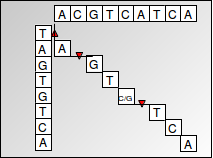
Figure 3.1: Global Alignment

To summarize the Needleman-Wunsch algorithm for global alignment:

We compute scores corresponding to each cell in the matrix and record our choice (memoization) at that step i.e. which one of the top, left or diagonal cells led to the maximum score for the current cell. We are left with a matrix full of optimal scores at each cell position, along with pointers at each cell reflecting the optimal choice that leads to that particular cell.

We can then recover the optimal alignment by tracing back from the cell in the bottom right corner (which contains the score of aligning one complete sequence with the other) by following the pointers reflecting locally optimal choices, and then constructing the alignment corresponding to an optimal path followed in the matrix.

The runtime of Needleman-Wunsch algorithm is O(n2) since for each cell in the matrix, we do a finite amount of computation. We calculate 3 values using already computed scores and then take the maximum of those values to find the score corresponding to that cell, which is a constant time (O(1)) operation.

To guarantee correctness, it is necessary to compute the cost for every cell of the matrix. It is possible that the optimal alignment may be made up of a bad alignment (consisting of gaps and mismatches) at the start, followed by many matches, making it the best alignment overall. These are the cases that traverse the boundary of our alignment matrix. Thus, to guarantee the optimal global alignment, we need to compute every entry of the matrix.

Global alignment is useful for comparing two sequences that are believed to be homologous. It is less useful for comparing sequences with rearrangements or inversions or aligning a newly-sequenced gene against reference genes in a known genome, known as database search. In practice, we can also often restrict the alignment space to be explored if we know that some alignments are clearly sub-optimal.

This chapter will address other forms of alignment algorithms to tackle such scenarios. It will first intro- duce the Smith-Waterman algorithm for local alignment for aligning subsequences as opposed to complete sequences, in contrast to the Needleman-Wunsch algorithm for global alignment. Later on, an overview will be given of hashing and semi-numerical methods like the Karp-Rabin algorithm for finding the longest (contiguous) common substring of nucleotides. These algorithms are implemented and extended for inexact matching in the BLAST program, one of the most highly cited and successful tools in computational biology. Finally, this chapter will go over BLAST for database searching as well as the probabilistic foundation of sequence alignment and how alignment scores can be interpreted as likelihood ratios.

Outline:

1. Introduction

   • Review of global alignment (Needleman-Wunsch)

2. Global alignment vs. Local alignment vs. Semi-global alignment
   • Initialization, termination, and update rules for Global alignment (Needleman-Wunsch) vs. Local alignment (Smith-Waterman) vs. Semi-global alignment
   • Varying gap penalties, algorithmic speedups
3. Linear-time exact string matching

   • Karp-Rabin algorithm and semi-numerical methods • Hash functions and randomized algorithms

4. The BLAST algorithm and inexact matching • Hashing with neighborhood search

   • Two-hit blast and hashing with combs

5. Pre-processing for linear-time string matching

   • Fundamental pre-processing
   • Suffix Trees
   • Suffix Arrays
   • The Burrows-Wheeler Transform

6. Probabilistic foundations of sequence alignment • Mismatch penalties, BLOSUM and PAM matrices

   • Statistical significance of an alignment score