2.8: Appendix

Last updated
Save as PDF

Page ID: 40918

\( \newcommand{\vecs}[1]{\overset { \scriptstyle \rightharpoonup} {\mathbf{#1}} } \) \( \newcommand{\vecd}[1]{\overset{-\!-\!\rightharpoonup}{\vphantom{a}\smash {#1}}} \)\(\newcommand{\id}{\mathrm{id}}\) \( \newcommand{\Span}{\mathrm{span}}\) \( \newcommand{\kernel}{\mathrm{null}\,}\) \( \newcommand{\range}{\mathrm{range}\,}\) \( \newcommand{\RealPart}{\mathrm{Re}}\) \( \newcommand{\ImaginaryPart}{\mathrm{Im}}\) \( \newcommand{\Argument}{\mathrm{Arg}}\) \( \newcommand{\norm}[1]{\| #1 \|}\) \( \newcommand{\inner}[2]{\langle #1, #2 \rangle}\) \( \newcommand{\Span}{\mathrm{span}}\) \(\newcommand{\id}{\mathrm{id}}\) \( \newcommand{\Span}{\mathrm{span}}\) \( \newcommand{\kernel}{\mathrm{null}\,}\) \( \newcommand{\range}{\mathrm{range}\,}\) \( \newcommand{\RealPart}{\mathrm{Re}}\) \( \newcommand{\ImaginaryPart}{\mathrm{Im}}\) \( \newcommand{\Argument}{\mathrm{Arg}}\) \( \newcommand{\norm}[1]{\| #1 \|}\) \( \newcommand{\inner}[2]{\langle #1, #2 \rangle}\) \( \newcommand{\Span}{\mathrm{span}}\)\(\newcommand{\AA}{\unicode[.8,0]{x212B}}\)

Homology

One of the key goals of sequence alignment is to identify homologous sequences (e.g., genes) in a genome. Two sequences that are homologous are evolutionarily related, specifically by descent from a common ancestor. The two primary types of homologs are orthologous and paralogous (refer to Figure 2.14¹¹). Other forms of homology exist (e.g., xenologs), but they are outside the scope of these notes.

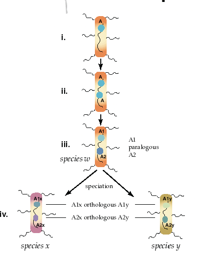
Figure 2.14: Ortholog and paralog sequences © source unknown. All rights reserved. This content is excluded from our Creative Commons license. For more information, see http://ocw.mit.edu/help/faq-fair-use/.

Orthologs arise from speciation events, leading to two organisms with a copy of the same gene. For example, when a single species A speciates into two species B and C, there are genes in species B and C that descend from a common gene in species A, and these genes in B and C are orthologous (the genes continue to evolve independent of each other, but still perform the same relative function).

Paralogs arise from duplication events within a species. For example, when a gene duplication occurs in some species A, the species has an original gene B and a gene copy B′, and the genes B and B′ are paralogus. Generally, orthologous sequences between two species will be more closely related to each other than paralogous sequences. This occurs because orthologous typically (although not always) preserve function over time, whereas paralogous often change over time, for example by specializing a gene’s (sub)function or by evolving a new function. As a result, determining orthologous sequences is generally more important than identifying paralogous sequences when gauging evolutionary relatedness.

Natural Selection

The topic of natural selection is a too large topic to summarize effectively in just a few short paragraphs; instead, this appendix introduces three broad types of natural selection: positive selection, negative selection, and neutral selection.

Positive selection occurs when a trait is evolutionarily advantageous and increases an individual’s fitness, so that an individual with the trait is more likely to have (robust) offspring. It is often associated with the development of new traits.
Negative selection occurs when a trait is evolutionarily disadvantageous and decreases an individual’s fitness. Negative selection acts to reduce the prevalence of genetic alleles that reduce a species’ fitness. Negative selection is also known as purifying selection due to its tendency to ’purify’ genetic alleles until only the most successful alleles exist in the population.
Neutral selection describes evolution that occurs randomly, as a result of alleles not affecting an indi- vidual’s fitness. In the absence of selective pressures, no positive or negative selection occurs, and the result is neutral selection.

Dynamic Programming v. Greedy Algorithms

Dynamic programming and greedy algorithms are somewhat similar, and it behooves one to know the distinctions between the two. Problems that may be solved using dynamic programming are typically optimization problems that exhibit two traits: 1. optimal substructure and 2. overlapping subproblems.

Problems solvable by greedy algorithms require both these traits as well as (3) the greedy choice property. When dealing with a problem “in the wild,” it is often easy to determine whether it satisfies (1) and (2) but difficult to determine whether it must have the greedy choice property. It is not always clear whether locally optimal choices will yield a globally optimal solution.

For computational biologists, there are two useful points to note concerning whether to employ dynamic programming or greedy programming. First, if a problem may be solved using a greedy algorithm, then it may be solved using dynamic programming, while the converse is not true. Second, the problem structures that allow for greedy algorithms typically do not appear in computational biology.

To elucidate this second point, it could be useful to consider the structures that allow greedy programming to work, but such a discussion would take us too far afield. The interested student (preferably one with a mathematical background) should look at matroids and greedoids, which are structures that have the greedy choice property. For our purposes, we will simply state that biological problems typically involve entities that are highly systemic and that there is little reason to suspect sufficient structure in most problems to employ greedy algorithms.

Pseudocode for the Needleman-Wunsch Algorithm

The first problem in the first problem set asks you to finish an implementation of the Needleman-Wunsch (NW) algorithm, and working Python code for the algorithm is intentionally omitted. Instead, this appendix summarizes the general steps of the NW algorithm (Section 2.5) in a single place.

Problem: Given two sequences S and T of length m and n, a substitution matrix vU of matching scores, and a gap penalty G, determine the optimal alignment of S and T and the score of the alignment.

Algorithm:

Create two m + 1 by n + 1 matrices A and B. A will be the scoring matrix, and B will be the traceback matrix. The entry (i, j) of matrix A will hold the score of the optimal alignment of the sequences S[1, . . . , i] and T [1, . . . , j], and the entry (i, j) of matrix B will hold a pointer to the entry from which the optimal alignment was built.
Initialize the first row and column of the score matrix A such that the scores account for gap penalties, and initialize the first row and column of the traceback matrix B in the obvious way.
Go through the entries (i, j) of matrix A in some reasonable order, determining the optimal alignment of the sequences S[1,...,i] and T[1,...,j] using the entries (i − 1,j − 1), (i − 1,j), and (i,j − 1). Set the pointer in the matrix B to the corresponding entry from which the optimal alignment at (i,j) was built.
Once all entries of matrices A and B are completed, the score of the optimal alignment may be found in entry (m, n) of matrix A.
Construct the optimal alignment by following the path of pointers starting at entry (m,n) of matrix B and ending at entry (0, 0) of matrix B.

¹¹ R.B. - BIOS 60579