2.1.2: Organizing Life on Earth

Learning Objectives

• Discuss the components and purpose of a phylogenetic tree.
• Interpret relationships between organisms using a phylogenetic tree.
• Correctly order the different levels of taxonomic classification.
• Discuss the benefits of having a comprehensive classification system.

The evolutionary history of a group of species is referred to as a phylogeny. Phylogeny describes the relationships of the group within the context of related organisms. Though phylogenetic relationships provide information on shared ancestry, they don't necessarily address how organisms are similar or different.

Phylogenetic Trees

Scientists use a tool called a phylogenetic tree to show the evolutionary pathways and connections among organisms. A phylogenetic tree is a diagram used to reflect evolutionary relationships among organisms or groups of organisms. Scientists consider phylogenetic trees to be a hypothesis of the evolutionary past since one cannot go back to confirm the proposed relationships. In other words, a “tree of life” can be constructed to illustrate when different organisms evolved and to show the relationships among different organisms (Figure \(\PageIndex{1}\)).

Unlike a taxonomic classification diagram, a phylogenetic tree can be read like a map of evolutionary history. Many phylogenetic trees have a single lineage at the base representing a common ancestor. Scientists call such trees rooted, which means there is a single ancestral lineage (typically drawn from the bottom or left) to which all organisms represented in the diagram relate. Notice in the rooted phylogenetic tree that the three domains— Bacteria, Archaea, and Eukarya—diverge from a single point and branch off. The small branch that plants and animals (indicated with a "you are here" star in Figure \(\PageIndex{1}\)) occupy in this diagram shows how recent and miniscule these groups are compared with other organisms. Unrooted trees don’t predict a common ancestor but do show relationships among species.

Figure \(\PageIndex{1}\): The phylogenetic tree in part a is rooted and resembles a living tree, with a common ancestor indicated as the base of the trunk. Two branches form from the trunk. The left branch leads to the domain Bacteria. The right branch branches again, giving rise to Archaea and Eukarya. Smaller branches within each domain indicate the groups present in that domain. The phylogenetic tree in part B is unrooted. It does not resemble a living tree; rather, groups of organisms within the Archaea, Eukarya, and Bacteria domains are arranged in a circle. Lines connect the groups within each domain. The groups within Archaea and Eukarya are then connected together. A line from the Archaea/Eukarya domains, and another from the Bacteria meet in the center of the circle. There is no root, and therefore no indication of which domain arose first. Both of these phylogenetic trees shows the relationship of the three domains of life—Bacteria, Archaea, and Eukarya—but the (a) rooted tree attempts to identify when various species diverged from a common ancestor while the (b) unrooted tree does not. (credit a: modification of work by Eric Gaba)

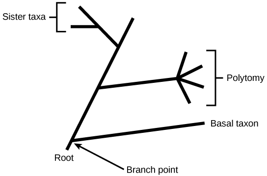
In a rooted tree, the branching indicates evolutionary relationships (see Figure \(\PageIndex{2}\)). The point where a split occurs, called a branch point or node, represents where a single lineage evolved into a distinct new one. A lineage that evolved early from the root and remains unbranched is called a basal taxon. When two lineages stem from the same branch point, they are called sister taxa. A branch with more than two lineages is called a polytomy and serves to illustrate where scientists have not definitively determined all of the relationships. It is important to note that although sister taxa and polytomy do share an ancestor, it does not mean that the groups of organisms split or evolved from each other. Organisms in two taxa may have split apart at a specific branch point, but neither taxa gave rise to the other.

Figure \(\PageIndex{2}\): The root of a phylogenetic tree indicates that an ancestral lineage gave rise to all organisms on the tree. A branch point indicates where two lineages diverged. A lineage that evolved early and remains unbranched is a basal taxon. When two lineages stem from the same branch point, they are sister taxa. A branch with more than two lineages is a polytomy. Descriptive text: A phylogenetic tree that starts at a root, indicating that all organisms on the tree share a common ancestor. Shortly after the root, the tree branches out. One branch gives rise to a single, basal lineage (basal taxon), and the other gives rise to all other organisms on the tree. The next branch forks at one point into four different lineages, an example of polytomy. The final branch gives rise to two lineages, an example of sister taxa.

The diagrams above can serve as a pathway to understanding evolutionary history. The pathway can be traced from the origin of life to any individual species by navigating through the evolutionary branches between the two points. By starting with a single species and tracing back towards the "trunk" of the tree, one can discover that species' ancestors, as well as where lineages share a common ancestry. In addition, the tree can be used to study entire groups of organisms.

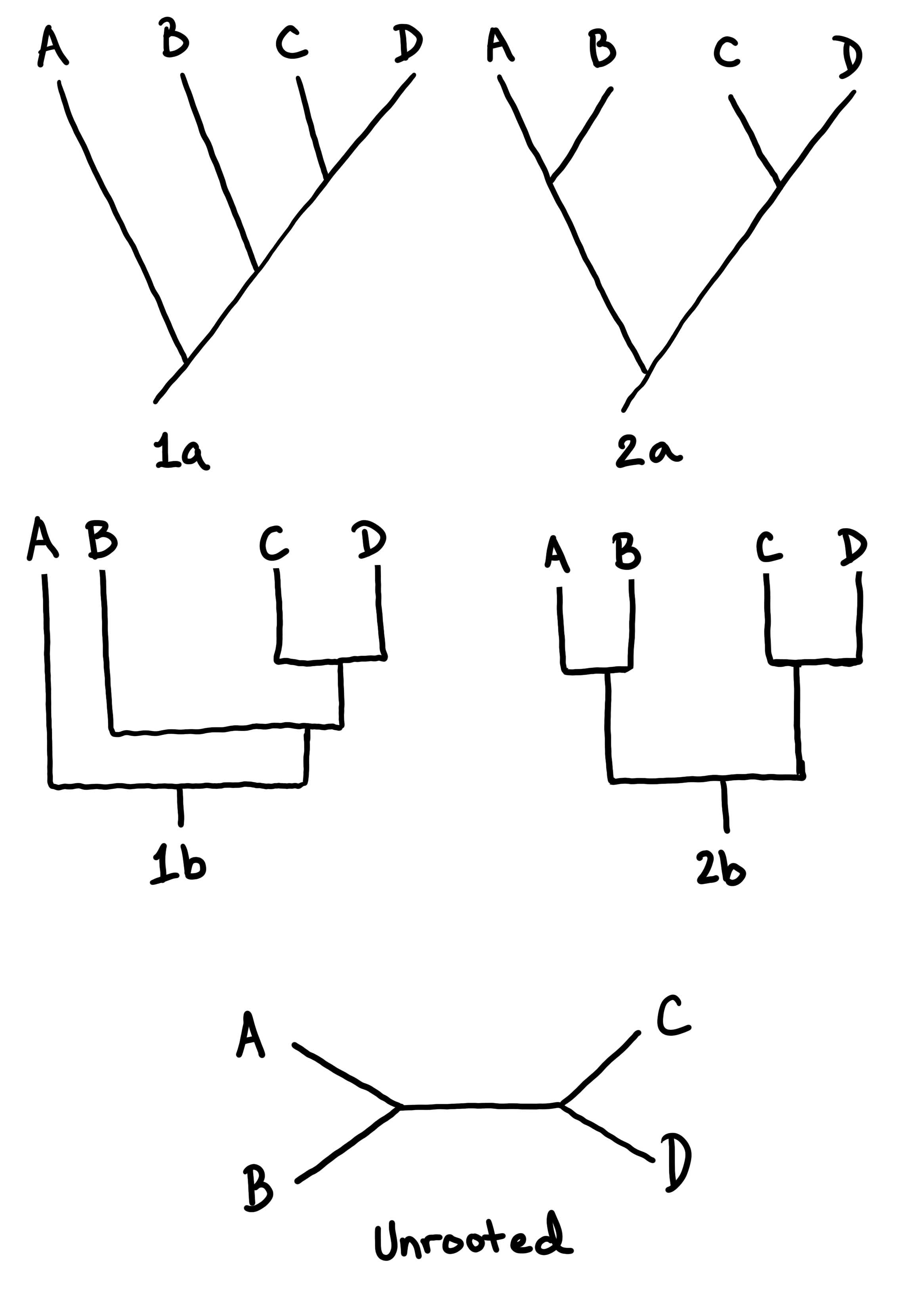
Another point to mention on phylogenetic tree structure is that rotation at branch points does not change the information. For example, if a branch point was rotated and the taxon order changed, this would not alter the information because the evolution of each taxon from the branch point was independent of the other.

Many disciplines within the study of biology contribute to understanding how past and present life evolved over time; these disciplines together contribute to building, updating, and maintaining the “tree of life.” Information is used to organize and classify organisms based on evolutionary relationships in a scientific field called systematics. Data may be collected from fossils, from studying the structure of body parts or molecules used by an organism, and by DNA analysis. By combining data from many sources, scientists can put together the phylogeny of an organism; since phylogenetic trees are hypotheses, they will continue to change as new types of life are discovered and new information is learned.

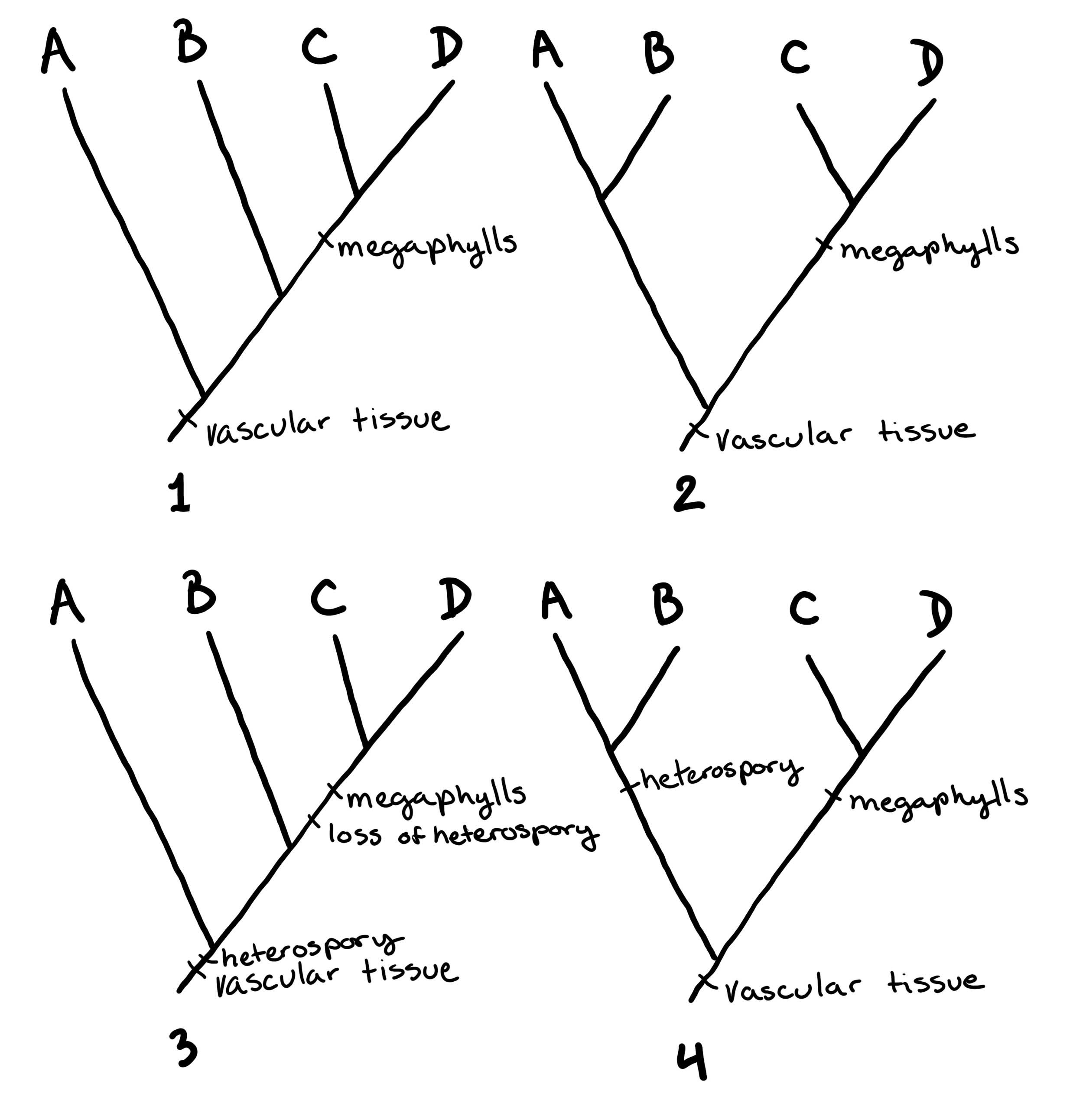
Examples of Simple Trees

In Figure \(\PageIndex{3}\) and Figure \(\PageIndex{4}\), some example trees are drawn to show how to interpret the structure of a phylogenetic tree.

Figure \(\PageIndex{3}\): These diagrams show hypotheses for four different taxa: A, B, C, and D. These taxa could represent individuals, different species, or any other level of classification. Trees 1a and 1b are drawn differently but represent the same hypothesis: C and D are most closely related (sister taxa) and A is the most ancestral lineage. Trees 2a and 2b represent a slightly different hypothesis: C and D are sister taxa, but A and B are also sister taxa; neither lineage is depicted as "older" than the other. This last relationship is also represented in the "Unrooted" tree: there is no hypothesis in this tree for which group is most ancestral (no "root"). Images drawn by Maria Morrow, CC-BY-NC.

Figure \(\PageIndex{4}\). Vascular tissue appears on the root of the trees as an ancestral trait. This means that A, B, C, and D all have vascular tissue. Megaphylls appears in both trees as a shared derived characteristic (synapomorphy) of C and D. This means C and D have megaphylls, but A and B do not. Both tree 1 and tree 2 are equally parsimonious. In trees 3 and 4, a third trait has been added: heterospory. In addition to the information from trees 1 & 2, we now see that A and B are heterosporous, while C and D are not. In tree 3, heterospory appears as an ancestral trait which is lost in C and D. In tree 4, heterospory is a synapomorphy of A and B. Tree 3 has four changes, while tree 4 only has three. This means that tree 4 is more parsimonious and therefore more likely (though not necessarily correct!). Images drawn by Maria Morrow, CC-BY-NC.

The Levels of Classification

Taxonomy (which literally means “arrangement law”) is the science of classifying organisms to construct internationally shared classification systems with each organism placed into more and more inclusive groupings. Think about how a grocery store is organized. One large space is divided into departments, such as produce, dairy, and meats. Then each department further divides into aisles, then each aisle into categories and brands, and then finally a single product. This organization from larger to smaller, more specific categories is called a hierarchical system.

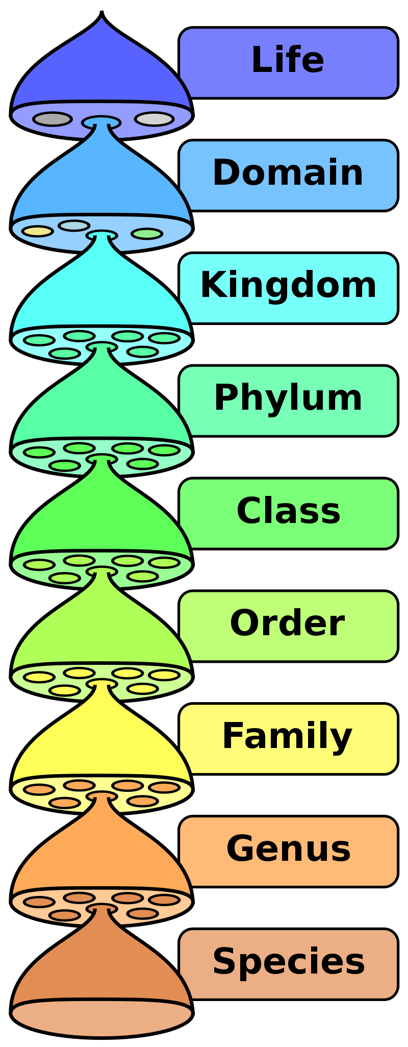
The taxonomic classification system (also called the Linnaean system after its inventor, Carl Linnaeus, a Swedish botanist, zoologist, and physician) uses a hierarchical model. Moving from the point of origin, the groups become more specific, until one branch ends as a single species. As you saw in Figure \(\PageIndex{1}\), scientists divide organisms into three large categories called domains: Bacteria, Archaea, and Eukarya. Within each domain is a second category called a kingdom. Each domain might encompass many kingdoms. For example, kingdom Plantae, kingdom Animalia, and kingdom Fungi represent three of the many kingdoms contained within domain Eukarya. After kingdoms, the subsequent categories of increasing specificity are: phylum, class, order, family, genus, and species (Figure \(\PageIndex{5}\)).

Figure \(\PageIndex{5}\): The taxonomic classification system uses a hierarchical model to organize living organisms into increasingly specific categories. Within what we have currently described as life, there are three domains. Within each domain, there are kingdoms. Within each kingdom, there are phyla. Within phyla there are classes, within classes there are orders, within orders there are families, within families there are genera, and within genera there are species. Diagram by Pengo, Public domain, via Wikimedia Commons.

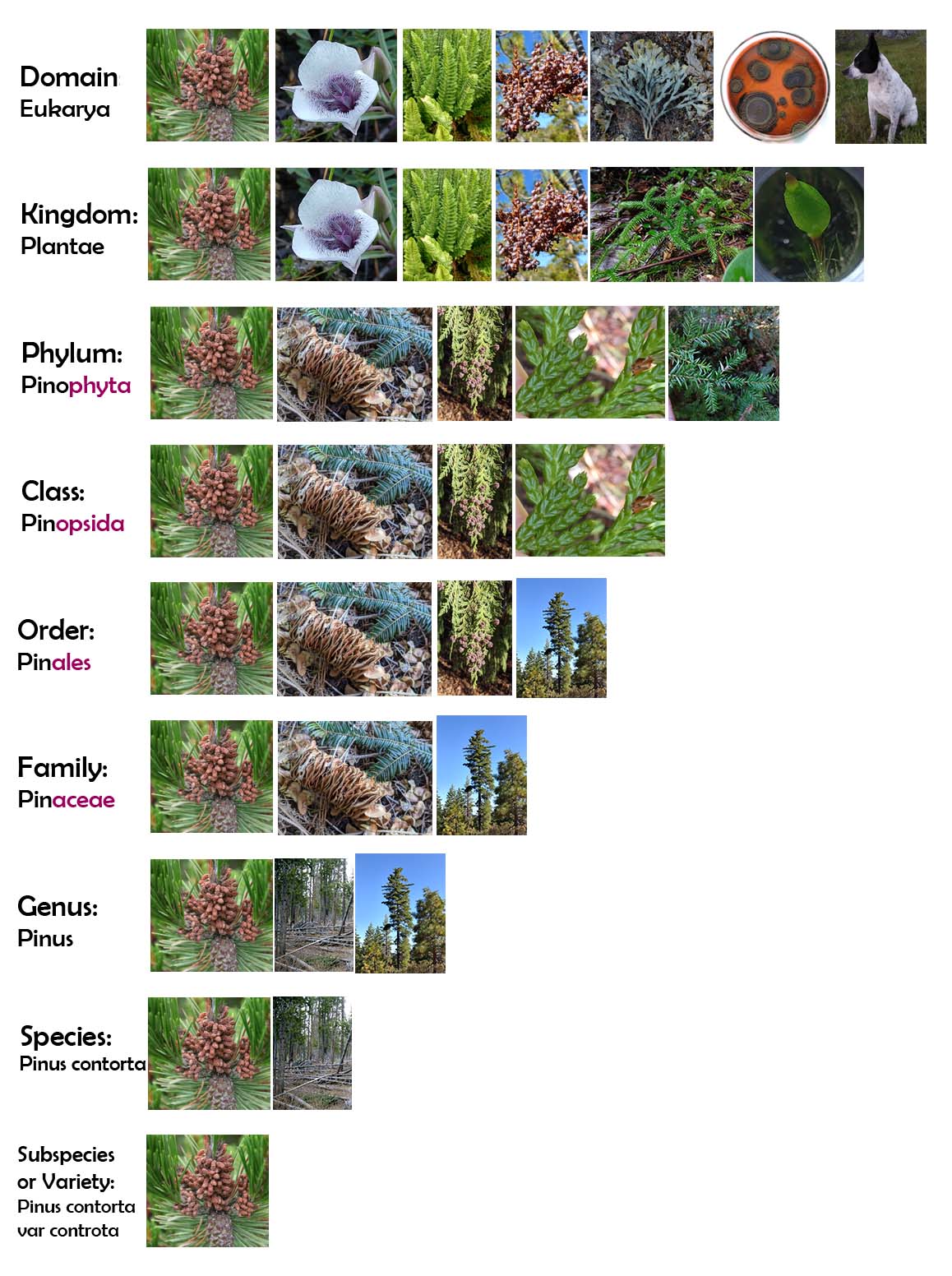
The kingdom Plantae stems from the Eukarya domain. For the shore pine (Pinus contorta var. contorta), the classification levels would be as shown in Figure \(\PageIndex{6}\). Therefore, the full name of an organism technically has multiple terms associated. For the shore pine, it is: Eukarya, Plantae, Pinophyta, Pinopsida, Pinales, Pinaceae, Pinus, Pinus contorta, and var. contorta. Notice that each name is capitalized except for the specific epithet (contorta), and the genus and species names are italicized. Notice also the underlined endings of the words. In plant taxonomy, the underlined portion is always used for those taxonomic levels: phyla end in -phyta, classes end in -opsida, orders end in -ales, and families end in -aceae.

The scientific name for an organism usually refers to the species name, a two-word scientific name that includes the genus name (e.g. Pinus) and specific epithet (e.g. contorta). This two word naming system is called binomial nomenclature. The name at each level is also called a taxon. In other words, pines are in order Pinales. Pinales is the name of the taxon at the order level; Pinaceae is the taxon at the family level, and so forth. Organisms also have a common name that people typically use, in this case, shore pine. Note that the shore pine is additionally a subspecies or variety: the second “contorta” in Pinus contorta var. contorta. Subspecies are members of the same species that are capable of mating and reproducing viable offspring, but they are considered separate subspecies due to geographic or behavioral isolation or other factors. Shore pines are coastal (hence the common name) and tend to grow in scraggly, twisted shapes (hence the scientific name). Lodgepole pines (Pinus contorta var. latifolia) typically have a straight trunk and grow in the mountains.

Figure \(\PageIndex{6}\) shows how the levels move toward specificity with other organisms. Notice how the shore pine (leftmost image) shares a domain with the widest diversity of organisms, including plants, fungi, algae, and animals. At each sublevel, the organisms become more similar because they are more closely related. Historically, scientists grouped similar organisms using characteristics, but as DNA technology developed, more precise relationships have been determined.

Figure \(\PageIndex{6}\): At each sublevel in the taxonomic classification system, organisms become more similar. Author's note: The reduction is slightly artificial in this diagram, as Pinales is the only order within Pinopsida. Figure and images by Maria Morrow, CC-BY-NC, except: the lodgepole pine, which comes from the public domain in the Wikimedia Commons, retrieved from the following page [1] of the Yellowstone Digital Slide Files archives; the Pinus contorta var contorta image, by Janice S, CC-BY-NC.

Recent genetic analysis and other advancements have found that some earlier phylogenetic classifications do not align with the evolutionary past; therefore, changes and updates must be made as new discoveries occur. Recall that phylogenetic trees are hypotheses and are modified as data becomes available. In addition, classification historically has focused on grouping organisms mainly by shared characteristics and does not necessarily illustrate how the various groups relate to each other from an evolutionary perspective. For example, despite the fact that a hippopotamus resembles a pig more than a whale, the hippopotamus may be the closest living relative of the whale.

Summary

Scientists continually gain new information that helps understand the evolutionary history of life on Earth. Each group of organisms went through its own evolutionary journey, called its phylogeny. Each organism shares relatedness with others, and based on morphologic and genetic evidence, scientists attempt to map the evolutionary pathways of all life on Earth. Historically, organisms were organized into a taxonomic classification system. However, today many scientists build phylogenetic trees to illustrate evolutionary relationships.

Contributors and Attributions

Curated and authored by Maria Morrow using the following sources:

• 20.1 Organizing Life on Earth from Biology by OpenStax (licensed CC-BY). Access for free at openstax.org.