1.1: Introduction

The Scientific Method

Scientists use a methodology for systematically investigating natural phenomena. This method uses existing information or observations to acquire new information or validate previous knowledge. These knowledge types come from empirical (experiential) or measured information. Empirical and measured data (or knowledge) are referred to as observations. While empirical data comes from experiences, science has developed into a mode of inquiry using experimentation. Experimental science uses the pre-existing base of knowledge to ask a testable question called a hypothesis. As a youngster, we’re incorrectly taught that a hypothesis is an educated guess. Formulating previous observations and measurements into a cohesive line of inquiry requires no guessing. People often have “theories” on something, when they actually have hypotheses based on their observations and assumptions.

Experimental Science

Hypothesis testing is the means by which experimental science is conducted. Experimental science is designed to enhance the understanding of a problem and removing biases from the interpretation. The goal of hypothesis testing is to try every way possible to disqualify the validity of the hypothesis. By doing so, the experimenter removes any biases in the experimental design. If the experimenter is unable to invalidate the hypothesis, the hypothesis becomes more valid and better able to act as a predictor of phenomena.

Experiments utilize controls. In a controlled experiment, there is a positive and negative control. These controls act as references in the experiment. A positive control is an experimental condition where the expected outcome that is tested will be produced. This control is necessary to assess the validity of a test or treatment. There can be multiple instances used as a positive control to examine the sensitivity of the experiment. A negative control is an experimental condition where the expected outcome is known not to occur. This type of control sometimes comes in the form of a sham or mock treatment such as giving someone a sugar pill (a placebo).

Through the use of experimental science and hypothesis testing, an increased refinement of existing knowledge can aid in designing new hypotheses. Hypothesis testing is re-iterative. That is to say, we use new knowledge to continue to enhance our understanding of the universe.

The scientific method is a reiterative process based on testing and revising knowledge. (CC-BY-NC-SA Jeremy Seto)

Theories

A scientific theory comes from repeated substantiation of multiple tested hypotheses. That is to say, confirmed hypotheses, observations, and experiments permit scientists to formulate a cohesive idea that integrates multiple substantiated pieces of evidence. As with hypotheses, theories are designed to be predictive and falsifiable. In the common language, we often hear the word theory to mean a conjecture, and as already discussed, conjectures based on evidence can be formulated into testable hypotheses.

When a theory is accepted by a predominant population of the specialists, it is referred to as a scientific principle. An example of a scientific principle is the theory of evolution by natural selection. Numerous tested hypotheses have been confirmed that lead to the understanding of natural selection as a method of evolution. This theory allows scientists to understand the underlying relatedness of all living things on the planet. Additionally, it unifies the disparate fields of Biology that can utilize the theory in a predictive manner. It is therefore also referred to as a unifying principle of Biology.

Classification of Life

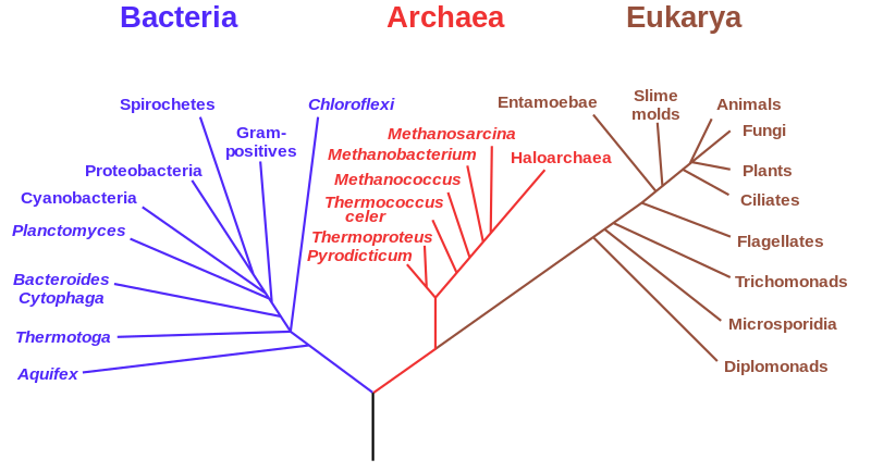
All living things on Earth share a relationship. The rules that govern life processes can be generalized across all organisms (living things), as well as non-living biological entities (viruses). The relatedness of organisms is often visualized as a phylogenetic tree. This tree is a hierarchical classification system that groups organisms together based on common features and used these similarities to name them. This is referred to as taxonomy with the broadest category is called a domain.

The phylogenetic tree of life describing the inter-relatedness of all living things on Earth.

Three domains exist, Archaea, Bacteria, and Eukarya. Archaea and Bacteria are also grouped together as Prokaryotes (pro– before; karya– nucleus). Eukarya (eu– true; karya– nucleus), or eukaryotes, is a group of organisms that have nuclei. The second most inclusive or broad category is Kingdom. Humans are in the Kingdom of animals. The third most inclusive or broad category is Phylum. Humans are in the phylum called Chordata. Each level of organization can be further subdivided and you may be more familiar with the subphylum called Vertebrata. Within this division, humans fall in the class of mammals. Amongst the mammals, humans are in the order of primates. Humans are categorized into a narrower group of organisms in the family of great apes or hominids. Within this family, humans fall into the genus of Homo. Biologists use a method of identifying specific organisms called binomial nomenclature. Binomial nomenclature uses the most specific groupings of taxonomy (genus and species) as a two-part name. While humans are of the species sapiens, the species name of humans using binomial nomenclature is Homo sapiens.

Taxonomic ranking of the red fox illustrating the inclusiveness of Domain and the exclusiveness of the Species level of categorization.

Credit: Annina Breen (CC-BY-SA 4.0)