5.4: Enzyme Kinetics

Studying enzyme kinetics can not only tell us about the catalytic properties of a particular enzyme but can also reveal important properties of biochemical pathways. Thus, one can determine a standard rate-limiting reaction under a given set of conditions by comparing kinetic data for each enzyme in a biochemical pathway. But what else can we do with kinetic data?

5.4.1. Why Study Enzyme Kinetics?

Apart from its value in teaching us how an individual enzyme actually works, kinetic data has great clinical value. For example, if we know the kinetics of each enzyme in the biochemical pathway for the synthesis of a liver metabolite in a healthy person, we also know what normally the rate-limiting (slowest) enzyme in the pathway is. Consider a patient whose blood levels of this metabolite are higher than normal. Could this be because the normal rate-limiting reaction is no longer rate-limiting in the patient? Which enzyme in the patient, then, is newly rate-limiting? Is there a possible therapy that can be developed using this information?

One can ask similar questions of an alternate scenario in which a patient is producing too little of the metabolite. A cellular biochemical might deviate from “normal” levels for a variety of reasons:

• Viral and bacterial infection or environmental poisons: These can interfere with a specific reaction in a metabolic pathway; remedies depend on this information!
• Chronic illness resulting from mutational enzyme deficiencies: Treatments might include medications designed to enhance or to inhibit (as appropriate) enzyme activity.
• Genetic illness tied to metabolic deficiency: If a specific enzyme is the culprit, investigation of a pre- and/or postnatal course of treatment might be possible (e.g., medication or perhaps even gene therapy).
• Lifestyle changes and choices: These might include eating habits, usually remediated by a change in diet.
• Lifestyle changes brought on by circumstance rather than choice: These are changes due to aging. An all-too-common example is the onset of type 2 diabetes. This can be treated with medication and/or delayed by switching to a low-carb diet favoring hormonal changes that would improve proper sugar metabolism.

Knowing the rate-limiting reaction(s) in biochemical pathways can help us identify regulated enzymes. This in turn may lead to a remedy to correct a metabolic imbalance. As noted, ribozymes are RNA molecules that catalyze biochemical reactions; their kinetics can also be analyzed and classified. We will consider how enzymes are regulated later, when we discuss glycolysis, a biochemical pathway that most living things use to extract energy from nutrients. For now, let’s look at an overview of experimental enzyme kinetics.

5.4.2. How We Determine Enzyme Kinetics and Interpret Kinetic Data

In enzyme kinetic studies, the enzyme is considered to be a reactant, albeit one that is regenerated by the end of the reaction. The reaction begins when substrate is added to the enzyme. In enzyme kinetic studies, the concentration of the enzyme is held constant while reaction rates are measured, after different amounts of substrate are added. As a consequence, all catalyzed reactions will reflect saturation of the enzyme at high concentration of substrate. This is the basis of saturation kinetics illustrated in Figure 5.6.

Figure 5.6: Enzyme saturation occurs when all available enzymes in solution are bound to substrate(s). Saturation kinetics experiments measure catalytic rates at different substrate(s) concentrations. At high substrate concentrations the active sites of all the enzymes are occupied, i.e., enzyme is saturated with substrate (far right). Under these conditions the reaction occurs at its fastest rate.

In the illustration, the active sites on all the enzyme molecules are bound to substrate molecules at a high substrate concentration. Under these conditions, a catalyzed reaction is proceeding at its fastest. Let’s generate some kinetic data to see saturation in action. The experiment illustrated in Figure 5.7 will determine the kinetics of the conversion of substrate (S) to product (P) by an enzyme (E).

Figure 5.7: The test tubes shown in this experiment each contain the same concentration of enzyme. After adding different amounts of substrate(s) to each tube, rates of product formation near the start of the reaction are measured to determine the kinetics of the enzyme-catalyzed reaction.

A series of reaction tubes are set up, each containing the same concentrations of E ([E]) but different concentrations of S ([S]). The concentration of P ([P]) produced at different times (beginning just after the start of the reaction in each tube) is plotted to determine the initial rate of P formation for each [S] tested. Figure 5.8 is such a plot.

Figure 5.8: This graph plots the rate of product (P) formation at different substrate concentrations ([S]) while holding the enzyme concentration ([E]) constant, as described in the experimental protocol in Figure 5.7.

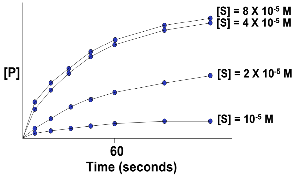
In this hypothetical example, the rates of the reactions (amounts of P made over time) do not increase beyond an [S] higher than \(4 \times 10^{-5}\)M. The upper curves thus represent the maximal rate of the reaction at the experimental concentration of enzyme. We say that the maximal reaction rate occurs at saturation.

CHALLENGE

What’s happening in this graph? Why do all the curves level off? Answer by imagining what the physical enzyme is doing at each point on the curves.

149 Measuring Enzyme Kinetics

Next, we can estimate the initial reaction rate (\(v_0\)) at each substrate concentration by plotting the slope of the first few time points through the origin of each curve in the graph. Consider the graph of the initial reaction rates estimated in this way in Figure 5.9 (below).

Figure 5.9: This graph shows the slopes (straight lines at the left) of the initial reaction rates taken from the curves in the previous graph (Figure 5.8). From the graph we can say that the enzyme became saturated somewhere between the two highest concentrations of substrate.

The slope of each straight line is the \(v_0\) for the reaction at a different [S] value near the very beginning of the reaction, when [S] is high and [P] is vanishingly low. Next, we plot these rates (slopes, or \(v_0\) values) against the different [S] values in the experiment to get the curve of the reaction kinetics in Figure 5.10.

Figure 5.10: This graph plots the initial reaction rates (slopes, or \(v_0\)) for the reactions plotted in Figure 5.9. The curve is approaching a maximum \(v_0\) (the asymptote at the right). The formula shown for this curve describes a rectangular hyperbola.

This is an example of Michaelis-Menten kinetics, which is common to many enzymes. Named after the biochemists who realized that the curve described rectangular hyperbola. Put another way, the equation mathematically describes the mechanism of catalysis of the enzyme!

The following equation mathematically describes a rectangular hyperbola:

\(y = \dfrac{\rm xa}{\rm x + b}\)

You might be asked to understand the derivation of the Michaelis-Menten equation in a biochemistry course. You might even be asked to do the derivation yourself! We won’t make you do that but suffice it to say that Michaelis and Menten started with some simple assumptions about how an enzyme-catalyzed reaction would proceed and then wrote reasonable chemical and rate equations for those reactions. The goal here is to understand those assumptions, to see how the kinetic data support those assumptions, and to realize what this tells us about how enzymes really work.

Here is one way to write the chemical equation for a simple reaction in which an enzyme (E) catalyzes the conversion of substrate (S) to product (P):

\(S \rightleftharpoons P\)

\(E\)

Michaelis and Menten rationalized that this reaction might actually proceed in three steps. In each step, enzyme E is treated as a reactant in the conversion of S to P. The resulting chemical equations are these:

\begin{aligned}
E + S &\rightleftharpoons E - S &&\text{binding of enzyme and substrate} \\
E - S &\rightleftharpoons E - P &&\text{conversion of substrate to product} \\
E - P &\rightleftharpoons E + P &&\text{dissociation of product and enzyme}
\end{aligned}

Reasoning that the middle reaction (the conversion of E and S to E and P) would be the fastest one and therefore would not be the rate-limiting reaction of catalysis, they only considered the first and third reactions to be relevant in determining the overall kinetics of product formation. Then they wrote the following rate equations for just these two chemical reactions (as one would in an introductory chemistry course):

\begin{aligned}
V_{\text{E-S formation}} &= k_1 [E][S] - k_{-1}[E-S] \\
V_{\text{P formation}} &= k_2[E-S] - k_{-2}[E][P]
\end{aligned}

Both of these equations describe a straight line. Therefore, neither describe the observed hyperbolic reaction kinetics. Finally, if you solve one of the equations for a term common to both (e.g., E-S) and then plug your solution into the other equation, your combined equation still describes described a straight line—again, not the expected rectangular hyperbola. To arrive at a chemical rate equation consistent with a rectangular hyperbola, Michaelis and Menten had to make several assumptions, including those made by G. E. Briggs and J. B. S. Haldane, about how E, S, and P would behave in a catalyzed reaction. Those assumptions allowed them to rewrite each equation, then to combine and to rewrite them into a single mathematical equation—one that did indeed describe a rectangular hyperbola. Here are Briggs and Haldane’s assumptions:

1. [S] >> [E] at the start and during the "steady state"
2. [P] << [S] at the start of a reaction.
3. All E is bound to S at the start of the reaction.
4. \([E]_{\rm total} = [E]_{\rm free} + [E-S]\) at all times.

We’ve already seen the equation that Michaelis and Menten derived from these assumptions, which is now known as the Michaelis-Menten equation:

\(V_0 = \dfrac{\rm Vmax[S]}{\rm Km + [S]}\)

The take-home message here is that the assumptions about an enzyme-catalyzed reaction are a good approximation of how the reaction proceeds over time. Michaelis and Menten defined Vmax and Km as key kinetic factors in enzyme-catalyzed reactions. In the generic example of substrate conversion to product, we saw that increasing [S] results in a higher rate of product formation because there is a higher rate of encounters between enzyme and substrate molecules. At some point, however, increasing [S] does not increase the initial reaction rate any further. Instead, \(v_0\) asymptotically approaches a theoretical maximum for the reaction, defined as Vmax, the maximum initial rate. As we have already seen, Vmax occurs when all available enzyme active sites are saturated (occupied by substrate). At this point, the intrinsic catalytic rate determines the turnover rate of the enzyme. The substrate concentration at which the reaction rate has reached ½ Vmax is defined as Km (the Michaelis-Menten constant), which is a ratio of the rate constants derived when rate equations for E-S and P formation (above) are rewritten and then combined into the single equation that describes a rectangular hyperbola.

150 Graphing Enzyme Kinetic Data

CHALLENGE

The Km is equivalent to a dissociation constant, while the reciprocal of the Km is often called the Ka, or affinity constant. Look carefully at the Michaelis-Menten curve and describe in words why the Km would be a measure of the tendency of enzyme and substrate to stay together (or conversely, to come apart).

To recapitulate, the two most important kinetic properties of an enzyme are the following:

1. The rate at which the enzyme becomes saturated with a particular substrate, which is related to the reaction’s Km
2. The maximum rate of the catalyzed reaction, which is described by the reaction’s Vmax

These properties suggest how an enzyme might behave under cellular conditions and can show how the enzyme should respond to allosteric regulation by natural inhibitory or activating factors, as well as how it might respond to poisons or other noxious chemicals.

For clear, detailed explanations of enzyme catalytic mechanisms, check out Jencks WP 1987, Catalysis in Chemistry and Enzymology Mineola, NY, Courier Dover Publications. You can also find more details of how kinetic equations are derived (an important step in understanding how the enzyme works) in any good biochemistry textbook, or you can check out the Michaelis-Menten Kinetics entry in the All About Enzymes Wikipedia link.