1.9: Evaluating the Ability of the ykkCD Toxin Sensor to Recognize the Antibiotic Tetracycline Using Fluorescent Quenching

9.1 Learning Objective

The goal of the mini project was to identify elements in the toxin sensor that are essential to recognize the antibiotic tetracycline. You identified elements in the sensor that did not change throughout evolution (invariable blocks). You subjected them to the site-directed mutagenesis, modified the sequence of the toxin sensor DNA and made the mutated toxin sensor RNAs. During this lab you will evaluate how well this mutant sensor is able to recognize the antibiotic tetracycline. If the mutant sensor is still able to recognize tetracycline, it means that the mutated invariable block was not essential for sensory function. If however, the mutated sensor fails to recognize tetracycline, it means that the mutated invariable block was essential for sensory function. You will perform binding affinity assays using fluorescence quenching to evaluate the affinity of the mutant sensor toward tetracycline.

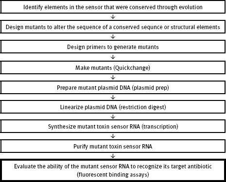
9.2 Mini Project Flowchart

The bolded block in the flowchart below highlights the role of the current experiment in the mini project.

9.3 What is Binding Affinity (K_D)?

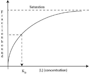
To estimate how well the mutated sensor RNA recognizes the antibiotic tetracycline, you will measure the binding affinity (K_D) of the tetracycline-sensor RNA complex. Binding affinity is the equilibrium dissociation constant. There is an inverse relationship between the strength of the interaction and the numeric value of the binding affinity: if the binding affinity is a small number, it means that addition of a small amount of RNA to tetracycline results in a high concentration of the sensor RNA-tetracycline complex. In other words, it only takes a small amount of tetracycline to form enough complex with the sensor RNA to trigger production of the efflux pump that in turn gets rid of tetracycline. Therefore, a small K_D value reflects a strong interaction between the antibiotic tetracycline and the sensor RNA. Likewise, a large K_D value reflects a week interaction between tetracycline and the sensor RNA. In other words if the K_D value is large, it takes a large amount of tetracycline to form enough tetracycline-RNA complex to trigger bacterial defense that gets rid of tetracycline. To measure binding affinity, one of the two reactants (tetracycline in our case) is kept at a constant low concentration while the concentration of the other reactant (sensor RNA) is varied. To determine the binding affinity, the fraction of tetracycline that is in complex with the sensor RNA is plotted against the RNA concentration. The dissociation constant is the sensor RNA concentration that forces 50% of tetracycline to form complex with the sensor RNA (Fig. 9).

Figure 9.1: The K_D value is the sensor RNA concentration that forces 50% of the tetracycline to form the tetracycline-ykkCD RNA complex.

9.4 What is Fluorescence?

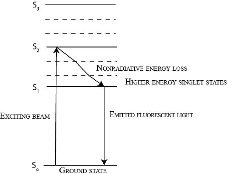
Fluorescence is a natural phenomenon. Some compounds, usually heterocyclic aromatic molecules, are able to absorb light of a specific energy and subsequently emit light that is lower in energy (larger wavelength) than the light absorbed. The wavelength of the light absorbed by the fluorescent compound is referred to as the excitation wavelength. The wavelength of the light emited by the fluorescent compound is referred to as the emission wavelength (Fig. 9.2).

Figure 9.2: Fluorescence is a natural phenomenon (top). Fluorescent compounds emit light that is lower in energy, and of higher wavelength, than the light absorbed (bottom).

During fluorescence, the incoming photons (excitation wave) excite electrons in the molecule to the higher energy excited states. The electrons lose some energy via nonradiative decay to reach the lowest energy excited state. From here, the excited electrons emit energy in form of photons (emission wave) to return to the ground state. The energy of the emission wave is lower than that of the excitation wave, because some energy was lost due to nonradiative decay, usually heat (Fig 9.3).

Figure 9.3: Jablonski diagram illustrates the electronic states of a molecule undergoing fluorescence. The electron is excited from the ground state to a higher energy excitation state. From there it releases energy through nonradiative decay then emits light (fluorescent light) to return to the ground state.

9.5 How Do We Measure Binding Affinity of the Tetracycline-Sensor RNA Complex?

To measure the binding affinity of the tetracycline-sensor RNA complex, you need to determine the fraction of tetracycline that is in complex with the toxin sensor RNA (fraction bound). To measure fraction bound you will take advantage of the natural fluorescence of tetracycline: once the sensor RNA forms a complex with tetracycline, the fluorescence of tetracycline decreases (quenching). The amount of quenching is proportional to the fraction of tetracycline that is bound to the sensor RNA (Fig 9.4).

Figure 9.4: Diagram of fluorescent binding assay. Once tetracycline is bound to the sensor its natural fluorescence decreases leading to fluorescent quenching.

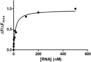
To determine the dissociation constant (K_D) you need to plot the amount of quenching (proportional to the fraction of tetracycline bound to the sensor RNA) against the sensor RNA concentration. This plot should shape as a hyperbola (saturation curve). Then you should fit the Equation 1 to determine the K_D value (Fig. 9.5).

Figure 9.5: Determination of K_D value. The amount of quenching is plotted against the sensor RNA concentration. The K_D value is the sensor RNA concentration where 50% of quenching is achieved.

9.6 How do We Evaluate Binding Affinity?

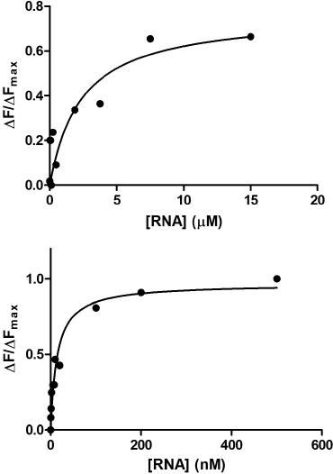
The goal of the mini-project was to identify parts of the toxin sensor that are essential for recognizing the antibiotic tetracycline. To reach the goal, you modified (mutated) evolutionary conserved parts of the toxin sensor and evaluated how well these mutated sensors were able to retain their ability to recognize tetracycline by measuring the K_D of the mutant sensor RNA-tetracycline complex. If the mutated sensor retain its ability to recognize tetracycline (small K_D value), the part of the sensor targeted for mutagenesis was not essential to recognize tetracycline. Likewise, if the mutated sensor lose its ability to recognize tetracycline (large K_D value), the part of the sensor targeted for mutagenesis was important for tetracycline recognition (Fig 9.6).

Figure 9.6: Schematics illustrating how to interpret the results of the binding affinity assays: Mutant 1 binds strongly to tetracycline, thus we conclude that the nucleotides changed were not essential for tetracycline recognition. In contrast, mutant 2 did not bind strongly to tetracycline. This means the nucleotides changed were probably important for tetracycline recognition.

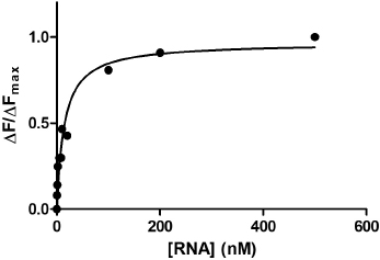
9.7 How do We Analyze Data?

Based on the data shown on Fig. 9.7, the mutant sensor-tetracycline complex has a K_D value of about a 100 nM. Compared to a binding affinity (10 nM) reported for the wild-type sensor RNA tetracycline complex, the mutant sensor slightly lost its ability to recognize the antibiotic tetracycline. Based on these data, we conclude that the part of the toxin sensor mutated is likely to be important for tetracycline recognition. To determine the K_D value of the mutant sensor-tetracycline complex more accurately, a higher mutant sensor RNA concentrations should be used in the future.

Figure 9.7: Example of data analysis. The binding affinity of the mutant sensor RNA-tetracycline complex is elevated (upper panel) compared to that of the wild-type sensor RNA tetracycline complex (lower panel). Elevated K_D value corresponds to weakened binding to tetracycline. Thus we conclude that the mutated nucleotides were important for tetracycline recognition.

What are we doing today?

1. Set up binding assays
2. Use demo data to fit binding curve and determine K_D

PROTOCOLS

Reagents and equipment needs are calculated per six student teams. There is ~20% excess included.

Equipment/glassware needed

1. Micropipettes 20-100 μl and 2-20 μl
2. Fluorescent plate reader
3. 96-well plates

Solutions needed

1. 5 x reaction buffer (100 mM Tris, pH=8.0; 500 mM KCl; 5 mM MgCl₂)
2. 20 nM tetracycline (in DMSO)
3. Ribolock RNase inhibitor (Fermentas, 40 U/μl)

Binding assay setup

Each student should set up 2 assays per mutant and one assay using the wild type ykkCD RNA sensor.

1. Prepare 2 solutions for each row (assay)

RNA containing solution

20 μl 5x reaction buffer

10 μl 20 nM tetracycline

Up to 70 μl or 1 μM final concentration sensor RNA

0.5 μl Ribonuclease inhibitor

Water to 100 μl if needed

No RNA solution

120 μl 5x reaction buffer

60 μl 20 nM tetracycline

3 μl Ribonuclease inhibitor

417 μl water

2. In each row perform serial dilution using the solutions above as follows

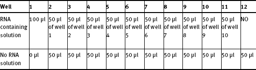
CALCULATE RNA CONCENTRATION OF EACH WELL ACCURATELY

4. Seal tray, cover with aluminum foil and incubate for 72 hrs. at 4 ºC.

Note to the instructor

The experiment in Chapter 9 was designed to determine the binding affinity of the mutant ykkCD sensor-tetracycline complex. The same protocol with minimal modifications can be used to measure binding affinity of any other fluorophore-macromolecule complex using fluorescent quenching. The binding assay worksheet may be incorporated into a lecture course that teaches binding affinity. 96-well plates used were manufactured by Corning Inc. (3991), but as long as the plates are black, flat bottom and have 96-wells, any other vendor might be used. Usage of RNase inhibitor is important to prevent RNA degradation especially considering the limited research experience of the experimenters. Assays may be read out by teaching assistants or by students that take the laboratory course at a different time of the week. A Tecan Infinite F200 plate reader was used to read out the assays; excitation wavelength was 380 nm, emission wavelength was 535 nm.

Analysis of Binding Experiments

In a common binding experiment to a set amount of one reagent (A) successive amounts of a second reagent (B) are added; the fractional amount bound (AB) is then measured. Since the second reagent (B) is added until all the first reagent (A) is bound, A is said to be “saturated” with B. Often the goal of the experiment is to determine the dissociation equilibrium constant, K_D.

Whether we study a binding protein or RNA, etc., the binding equilibrium can be treated in the same way:

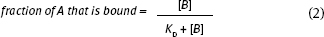
Equation 2 predicts a hyperbolic binding curve (see below). This is sometimes termed a “saturation” curve because A is finally saturated with B.

Figure 9.8: Saturation curve depicting binding of a ligand to a receptor. K_D value indicates the ligand concentration at which the binding site on a particular protein is half occupied.

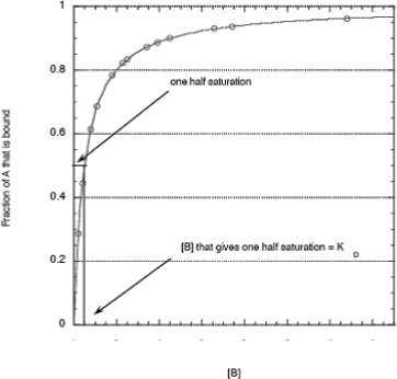
The dissociation equilibrium constant is equal to the concentration of B that gives one half-saturation. For the RNA sensor binding assay, you will use a set amount of tetracycline to which increasing amounts of RNA will be added. The fluorescence of tetracycline will decrease as it is bound by the RNA.

Fluorescent quenching is used to measure the fraction of tetracycline bound by RNA.

where

and

Figure 9.9: Saturation curve depicting binding of tetracycline to the sensor RNA. K_D value indicates the ligand concentration where 50% of the sensor RNA is bound with tetracycline.

The RNA-Tetracycline Binding Worksheet contains problems that allow you to work through these calculations.

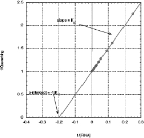
Once you have plotted the hyperbolic binding curve, you need to use a double reciprocal plot; this generally gives a better measure of K_D. The reciprocal of the binding equation predicts a straight line plot:

Figure 9.10: Linear representation of a saturation curve. The K_D value may be determined in two different ways: (1) the slope of the graph equals the K_D value or (b) the x-intercept is -1/K_D.

Binding Assays Prelab

Work with the following data from binding assays using two sensor RNA mutants. Please use a computer graphing program. Mutations are highlighted on the figure below.

Figure 9.11: B. subtilis ykkCD sensor RNA secondary structure: Color coding is as follows: red, 100% sequence conservation; blue, >80% sequence conservation and black, no significant sequence conservation.

1. (10 pts.) The fluorescence from tetracycline was measured as a function of [RNA] for Mutant #1 and the following results were obtained (Quenching = ΔFl/ΔFlmax):

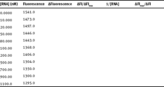
• a) Plot quenching versus [RNA] and estimate the K_D for tetracycline-RNA binding. Show how you estimated the dissociation constant.
  
  
  
  
  
  
• b) Use a double reciprocal plot to get a better estimate of K_D.

2. (15 pts.) Mutant #2 was also studied. The stock [RNA] was 2.4 × 10^-5 M. The procedure for this experiment matched the one you are running in lab. Prepare a double reciprocal plot and determine the K_D for mutant #2.

3. (5 pts.) Which mutation has a larger impact on tetracycline binding? Briefly explain.

Lab Report Outline and Point Distribution

1. Several sentences defining the goal/purpose of each procedure. Describe the role this step plays in the mini project (5 pts.).

2. Describe fluorescence (about five sentences; 5 pts.).

3. Show an example of your calculations for RNA concentration in the binding assay (3 pts.).

4. Use a computer to plot (20 pts. total):

• a. Quenching vs. [RNA] for each assay; determine the K_D from the curves. Report error and standard deviation!
• b. 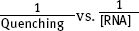for each assay; determine the K_D from these double reciprocal plots. Report error and standard deviation!
• c. Do you consider your K_D measurement reliable? Briefly explain. How would you modify your experiment to more accurately determine K_D? For example, could you change the [RNA] range? Briefly explain (10 pts.).

5. In your judgment how did the mutation affect the ability of the sensor to recognize the antibiotic tetracycline? Do you think the mutated region was important for antibiotic recognition? How does the K_D of the mutant sensor – tetracycline complex relate to that of the wild type sensor - tetracycline complex? (7 pts.).