3.20: 2020_Winter_Bis2a_Facciotti_Lecture_19

Learning objectives associated with 2020_Winter_Bis2a_Facciotti_Lecture_19 Describe a genome as the complete collection of heritable nucleotides whose sequence can be increasingly quickly and inexpensively determined and annotated with rapidly evolving instrumentation (micro and nano) and computational technologies. Describe the diversity of features (e.g. coding, non-coding, repeat) found in genomes of different organisms and the different densities and frequencies with which different kinds of features may be found. Propose reasonable hypotheses for why different genomes may be more or less densely packed with identifiable genetic features.

 

Genomes as organismal blueprints

A genome is an organism's complete collection of heritable information stored in DNA. Differences in information content help to explain the diversity of life we see all around us. Changes to the information encoded in the genome are the primary drivers of the phenotypic diversity we see (and some we can't) around us that are filtered by natural selection, and they are thus the drivers of evolution. This leads to questions. If every cell in a multicellular organism contains the same sequence of DNA, how can there be different cell types (e.g., how can a cell in a liver be so different from a cell in the brain if they both carry the same DNA)? How do we read the information? How do we interpret what we read? How do we understand how all the "parts" we identify in the genome functionally interrelate? How is all of this related to the expression of traits? How do changes in the genome lead to changes in traits?

Determining a genome sequence

The information encoded in genomes provides important data for understanding life, its functions, its diversity, and its evolution. Therefore, a reasonable place to begin studies in biology would be to read the information content encoded in the genome(s) in question. A good starting point is to determine the sequence of nucleotides (A, G, C, T) and their organization into one or more independently replicating units of DNA (e.g., think chromosomes and/or plasmids ). For 30+ years after the discovery that DNA is the hereditary material, this was a daunting proposition. In the late 1980s, however, the advent of semi-automated tools for DNA sequencing were pioneered, and this began a revolution that has dramatically changed how we approach the study of life. Twenty years later, in the mid-2000s, we entered a period of accelerated technological progress in which advances in materials sciences (particularly, advances in our ability to make things on a tiny scale), optics, electrical and computer engineering, bioengineering, and computer sciences have all converged to bring us dramatic increases in our capacity to sequence DNA and correspondingly dramatic decreases in the cost of sequencing DNA. A famous example to illustrate this point is to compare the changes in cost to sequence the human genome. The first draft of the human genome took nearly 15 years and $3 billion dollars to complete. Today, 10's of human genomes can be sequenced in a single day on a single instrument at a cost of less than $1000 each (the cost and time continue to decrease). Today, companies like Illumina, Pacific Biosciences, Oxford Nanopore, and others offer competing technologies that are driving down the cost and increasing the volume, quality, speed, and portability of DNA sequencing.

One of the very exciting elements of the DNA sequencing revolution is that it has required and continues to require contributions from biologists, chemists, materials scientists, electrical engineers, mechanical engineers, computer scientists and programmers, mathematicians and statisticians, product developers, and many other technical experts. The potential applications and implications of unlocking barriers to DNA sequencing have also engaged investors, business people, product developers, entrepreneurs, ethicists, policy makers, and many others to pursue new opportunities and to think about how to best and most responsibly use this growing technology.

The technological advances in genome sequencing have resulted in a virtual flood of complete genome sequences being determined and deposited into publicly available databases. You can find many of them at the National Center for Biotechnology Information. The number of available, completely sequenced genomes numbers in the tens of thousands—over 2,000 eukaryotic genomes, over 600 archaeal genomes, and nearly 12,000 bacterial genomes at the time of this writing. Tens of thousands of additional genome sequencing projects are in progress. With this many genome sequences available—or soon to be available—we can start asking many questions about what we see in these genomes. What patterns are common to all genomes? How many genes are encoded in genomes? How are these organized? How many types of features can we find? What do the features we find do? How different are the genomes from one another? Is there evidence that can tell us how genomes evolve? Let's briefly examine a few of these questions.

Diversity of genomes

Diversity of sizes, number of genes, and chromosomes

Let's start by examining the range of genome sizes. In the table below, we see a sampling of genomes from the database. We can see that the genomes of free-living organisms range tremendously in size. The smallest known genome is encoded by 580,000 base pairs while the largest is 150 billion base pairs—for reference, recall that the human genome is 3.2 billion base pairs. That's a huge range of sizes. Similar disparities in the number of genes also exist.

Table 1. This table shows some genome data for various organisms. 2n = diploid number. Attribution: Marc T. Facciotti (own work—reproduced from http://book.bionumbers.org/how-big-are-genomes/)

 

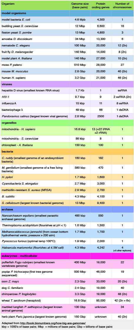
Examining Table 1 also reveals that some organisms carry with them more than one chromosome. Some genomes are also polyploid, meaning that they maintain multiple copies of similar but not identical (homologous) copies of each chromosome. A diploid organism carries in its genome two homologous copies (usually one from Mom and one from Dad) of each chromosome. Humans are diploid. Our somatic cells carry 2 homologous copies of 23 chromosomes. We received 23 copies of individual chromosomes from our mother and 23 copies from our father, for a total of 46. Some plants have a higher ploidy. For example, we term a plant with four homologous copies of each chromosome tetraploid. We term an organism with a single copy of each chromosome haploid.

Structure of genomes

Table 1 also provides clues to other points of interest. For instance, if we compare the pufferfish genome to the chimpanzee genome, we note that they encode roughly the same number of genes (19,000), but they do so on dramatically differently sized genomes—400 million base pairs versus 3.3 billion base pairs, respectively. That implies that the pufferfish genome must have much less space between its genes than what we might expect to find in the chimpanzee genome. This is the case, and the difference in gene density is not unique to these two genomes. If we look at Figure 1, which attempts to represent a 50-kb part of the human genome, we notice that besides the protein-coding regions (indicated in red and pink) that many other so-called "features" can be read from the genome. Many of these elements contain highly repetitive sequences.

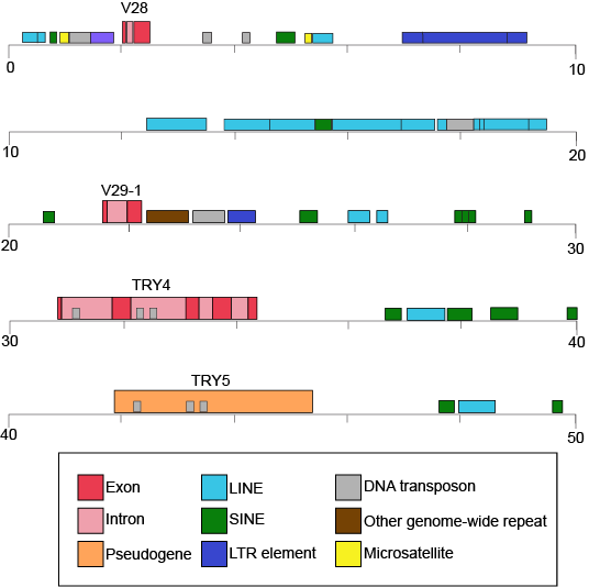
Figure 1. This figure shows a 50-kb segment of the human β T-cell receptor locus on chromosome 7. This figure depicts a small region of the human genome and the types of "features" that can be read and decoded in the genome, including, but also besides, protein-coding sequences. Red and pink correspond to regions that encode proteins. Other colors represent different types of genomic elements. Attribution: Marc T. Facciotti (own work—reproduced from www.ncbi.nlm.nih.gov/books/NBK21134/)

If we now look at what fraction of the whole human genome each of these types of elements makes up (see Figure 2), we see that protein-coding genes only make up 48 million of the 3.2 billion bases of the haploid genome.

 

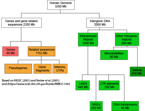
Figure 2. This graph depicts how the many base pairs of DNA in the human haploid genome are distributed between various identifiable features. Note that only a small fraction of the genome is associated directly with protein-coding regions. Attribution: Marc T. Facciotti (own work—reproduced from sources noted in figure)

 

When we examine the frequency of repeat regions versus protein-coding regions in different species, we note large differences in protein-coding versus non-coding regions.

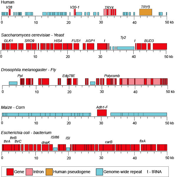
Figure 3. This figure shows 50-kb segments of different genomes, illustrating the highly variable frequency of repeat versus protein-coding elements in different species.
Attribution: Marc T. Facciotti (own work—reproduced from www.ncbi.nlm.nih.gov/books/NBK21134/)

 

---

Possible NB Discussion Point

Propose a hypothesis for why you think some genomes might have more or fewer noncoding sequences.

---

 

Dynamics of genome structure

Genomes change over time, and many events can change their sequence.

1. Mutations are accumulated during DNA replication or through environmental exposure to chemical mutagens or radiation. These changes typically occur at the level of single nucleotides.
2. Genome rearrangements describe a class of large-scale changes that can occur, and they include: (a) deletions—where segments of the chromosome are lost; (b) duplication—where regions of the chromosome are inadvertently duplicated; (c) insertions—the insertion of genetic material (note that sometimes this is acquired from viruses or the environment, and deletion/insertion pairs may happen across chromosomes); (d) inversions—where regions of the genome are flipped within the same chromosome; and (e) translocations—where segments of the chromosome are translocated (moved elsewhere in the chromosome).

These changes happen at different rates, and some are facilitated by the activity of enzyme catalysts (e.g., transposases).

 

---

Possible NB Discussion Point

How might mutations and genome rearrangements complicate studying/analyzing genomes? Conversely, can you think of interesting questions we can ask by comparing variation between genomes that occur because of events like mutation and genome rearrangements?

---

 

The study of genomes

Comparative genomics

One of the most common things to do with a collection of genome sequences is to compare the sequences of multiple genomes to one another. In general terms, these types of activities fall under the umbrella of a field called comparative genomics.

Comparing the genomes of people who suffer from an inheritable disease to the genomes of people who are not afflicted can help us uncover the genetic basis for the malady. Comparing the gene content, order, and sequence of related microbes can help us find the genetic basis of why some microbes cause disease while their close cousins are virtually harmless. We can compare genomes to understand how a new species may have evolved. There are many possible analyses! The basis of these analyses is similar: look for differences across multiple genomes and try to associate those differences with different traits or behaviors in those organisms.

Last, some people are comparing genome sequences to understand the evolutionary history of the organisms. Typically, these types of comparisons result in a graph known as a phylogenetic tree, which is a graphical model of the evolutionary relationship between the various species being compared. This field, not surprisingly, is called phylogenomics.

Metagenomics: Who is living somewhere and what are they doing?

Besides studying the genomes of individual species, the increasingly powerful DNA-sequencing technologies are making it possible to sequence simultaneously the genomes of environmental samples inhabited by many species. This field is called metagenomics. These studies are typically focused on trying to understand what microbial species inhabit different environments. There is great interest in using DNA sequencing to study the populations of microbes in the gut and to watch how the population changes in response to different diets, to see if there is any association between the abundance of different microbes and various diseases, or to look for pathogens. People are using DNA sequencing of environmental metagenomic samples to explore which microbes inhabit different environments on Earth (from the deep sea, to soil, to air, to hypersaline ponds, to cat feces, to some common surfaces we touch every day).

Besides discovering "who lives where," the sequencing of microbial populations in different environments can also reveal what protein-coding genes are present in an environment. This can give investigators clues into what metabolic activities might occur in that environment. Besides providing important information about what kind of chemistry might happen in a specific environment, the catalog of genes that is accumulated can also serve as an important resource for the discovery of novel enzymes for applications in biotechnology.